Neural Save and Load Models

- skip_showdoc: true

Author

Benedict Thekkel

Saving and loading trained Deep Learning models has multiple valuable uses. These models are often costly to train; storing a pre-trained model can help reduce costs as it can be loaded and reused to forecast multiple times. Moreover, it enables Transfer learning capabilities, consisting of pre-training a flexible model on a large dataset and using it later on other data with little to no training. It is one of the most outstanding 🚀 achievements in Machine Learning 🧠 and has many practical applications.

In this notebook we show an example on how to save and load NeuralForecast models.

The two methods to consider are:
1. NeuralForecast.save: Saves models into disk, allows save dataset and config.
2. NeuralForecast.load: Loads models from a given path.

Important

This Guide assumes basic knowledge on the NeuralForecast library. For a minimal example visit the Getting Started guide.

You can run these experiments using GPU with Google Colab.

1. Installing NeuralForecast

%%capture !pip install neuralforecast

2. Loading AirPassengers Data

For this example we will use the classical AirPassenger Data set. Import the pre-processed AirPassenger from utils.

from neuralforecast.utils import AirPassengersDF

Y_df = AirPassengersDF
Y_df = Y_df.reset_index(drop=True)
Y_df.head()

	unique_id	ds	y
0	1.0	1949-01-31	112.0
1	1.0	1949-02-28	118.0
2	1.0	1949-03-31	132.0
3	1.0	1949-04-30	129.0
4	1.0	1949-05-31	121.0

3. Model Training

Next, we instantiate and train three models: NBEATS, NHITS, and AutoMLP. The models with their hyperparameters are defined in the models list.

from ray import tune

from neuralforecast.core import NeuralForecast
from neuralforecast.auto import AutoMLP
from neuralforecast.models import NBEATS, NHITS

horizon = 12
models = [NBEATS(input_size=2 * horizon, h=horizon, max_steps=50),
          NHITS(input_size=2 * horizon, h=horizon, max_steps=50),
          ]

Global seed set to 1
Global seed set to 1

nf = NeuralForecast(models=models, freq='M')
nf.fit(df=Y_df)

Produce the forecasts with the predict method.

Y_hat_df = nf.predict().reset_index()
Y_hat_df.head()

	unique_id	ds	NBEATS	NHITS
0	1.0	1961-01-31	446.280823	445.295135
1	1.0	1961-02-28	463.121948	462.276184
2	1.0	1961-03-31	470.079895	475.442902
3	1.0	1961-04-30	492.255310	503.250916
4	1.0	1961-05-31	535.243164	556.968689

We plot the forecasts for each model. Note how the two NBEATS models are differentiated with a numerical suffix.

import pandas as pd
import matplotlib.pyplot as plt

plot_df = pd.concat([Y_df, Y_hat_df]).set_index('ds') # Concatenate the train and forecast dataframes

plt.figure(figsize = (12, 3))
plot_df[['y', 'NBEATS', 'NHITS']].plot(linewidth=2)

plt.title('AirPassengers Forecast', fontsize=10)
plt.ylabel('Monthly Passengers', fontsize=10)
plt.xlabel('Timestamp [t]', fontsize=10)
plt.axvline(x=plot_df.index[-horizon], color='k', linestyle='--', linewidth=2)
plt.legend(prop={'size': 10})

<Figure size 1200x300 with 0 Axes>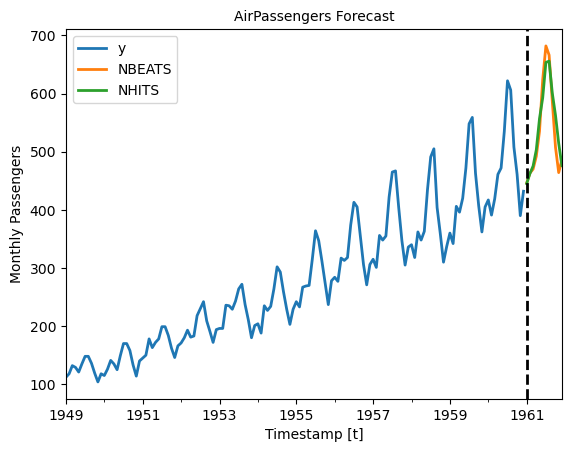

4. Save models

To save all the trained models use the save method. This method will save both the hyperparameters and the learnable weights (parameters).

The save method has the following inputs:

path: directory where models will be saved.
model_index: optional list to specify which models to save. For example, to only save the NHITS model use model_index=[2].
overwrite: boolean to overwrite existing files in path. When True, the method will only overwrite models with conflicting names.
save_dataset: boolean to save Dataset object with the dataset.

nf.save(path='./checkpoints/test_run/',
        model_index=None, 
        overwrite=True,
        save_dataset=True)

For each model, two files are created and stored:

[model_name]_[suffix].ckpt: Pytorch Lightning checkpoint file with the model parameters and hyperparameters.
[model_name]_[suffix].pkl: Dictionary with configuration attributes.

Where model_name corresponds to the name of the model in lowercase (eg. nhits). We use a numerical suffix to distinguish multiple models of each class. In this example the names will be automlp_0, nbeats_0, and nhits_0.

Important

The Auto models will be stored as their base model. For example, the AutoMLP trained above is stored as an MLP model, with the best hyparparameters found during tuning.

5. Load models

Load the saved models with the load method, specifying the path, and use the new nf2 object to produce forecasts.

nf2 = NeuralForecast.load(path='./checkpoints/test_run/')
Y_hat_df = nf2.predict().reset_index()
Y_hat_df.head()

Global seed set to 1
Global seed set to 1

	unique_id	ds	NHITS	NBEATS
0	1.0	1961-01-31	445.295135	446.280823
1	1.0	1961-02-28	462.276184	463.121948
2	1.0	1961-03-31	475.442902	470.079895
3	1.0	1961-04-30	503.250916	492.255310
4	1.0	1961-05-31	556.968689	535.243164

Finally, plot the forecasts to confirm they are identical to the original forecasts.

plot_df = pd.concat([Y_df, Y_hat_df]).set_index('ds') # Concatenate the train and forecast dataframes

plt.figure(figsize = (12, 3))
plot_df[['y', 'NBEATS', 'NHITS']].plot(linewidth=2)

plt.title('AirPassengers Forecast', fontsize=10)
plt.ylabel('Monthly Passengers', fontsize=10)
plt.xlabel('Timestamp [t]', fontsize=10)
plt.axvline(x=plot_df.index[-horizon], color='k', linestyle='--', linewidth=2)
plt.legend(prop={'size': 10})
plt.show()

<Figure size 1200x300 with 0 Axes>

References

https://pytorch-lightning.readthedocs.io/en/stable/common/checkpointing_basic.html

Oreshkin, B. N., Carpov, D., Chapados, N., & Bengio, Y. (2019). N-BEATS: Neural basis expansion analysis for interpretable time series forecasting. ICLR 2020

Cristian Challu, Kin G. Olivares, Boris N. Oreshkin, Federico Garza, Max Mergenthaler-Canseco, Artur Dubrawski (2021). N-HiTS: Neural Hierarchical Interpolation for Time Series Forecasting. Accepted at AAAI 2023.