This Guide assumes basic familiarity with StatsForecast. For a minimal example visit the Quick Start.
Follow this article for a step to step guide on building a production-ready forecasting pipeline for multiple time series.
During this guide you will gain familiary with the core StatsForecastclass and some relevant methods like StatsForecast.plot, StatsForecast.forecast and StatsForecast.cross_validation.
We will use a classical benchmarking dataset from the M4 competition. The dataset includes time series from different domains like finance, economy and sales. In this example, we will use a subset of the Hourly dataset.
We will model each time series individually. Forecasting at this level is also known as local forecasting. Therefore, you will train a series of models for every unique series and then select the best one. StatsForecast focuses on speed, simplicity, and scalability, which makes it ideal for this task.
Outline:
Install packages.
Read the data.
Explore the data.
Train many models for every unique combination of time series.
Evaluate the model’s performance using cross-validation.
Select the best model for every unique time series.
We assume you have StatsForecast already installed. Check this guide for instructions on how to install StatsForecast.
Read the data
We will use pandas to read the M4 Hourly data set stored in a parquet file for efficiency. You can use ordinary pandas operations to read your data in other formats likes .csv.
The input to StatsForecast is always a data frame in long format with three columns: unique_id, ds and y:
The unique_id (string, int or category) represents an identifier for the series.
The ds (datestamp or int) column should be either an integer indexing time or a datestampe ideally like YYYY-MM-DD for a date or YYYY-MM-DD HH:MM:SS for a timestamp.
The y (numeric) represents the measurement we wish to forecast. The target column needs to be renamed to y if it has a different column name.
This data set already satisfies the requirements.
Depending on your internet connection, this step should take around 10 seconds.
import pandas as pdY_df = pd.read_parquet('https://datasets-nixtla.s3.amazonaws.com/m4-hourly.parquet')Y_df
unique_id
ds
y
0
H1
1
605.0
1
H1
2
586.0
2
H1
3
586.0
3
H1
4
559.0
4
H1
5
511.0
...
...
...
...
373367
H99
744
24039.0
373368
H99
745
22946.0
373369
H99
746
22217.0
373370
H99
747
21416.0
373371
H99
748
19531.0
373372 rows × 3 columns
This dataset contains 414 unique series with 900 observations on average. For this example and reproducibility’s sake, we will select only 10 unique IDs and keep only the last week. Depending on your processing infrastructure feel free to select more or less series.
Note
Processing time is dependent on the available computing resources. Running this example with the complete dataset takes around 10 minutes in a c5d.24xlarge (96 cores) instance from AWS.
uids = Y_df['unique_id'].unique()[:10] # Select 10 ids to make the example fasterY_df = Y_df.query('unique_id in @uids') Y_df = Y_df.groupby('unique_id').tail(7*24) #Select last 7 days of data to make example fasterY_df
unique_id
ds
y
580
H1
581
587.0
581
H1
582
537.0
582
H1
583
492.0
583
H1
584
464.0
584
H1
585
443.0
...
...
...
...
7475
H107
744
4316.0
7476
H107
745
4159.0
7477
H107
746
4058.0
7478
H107
747
3971.0
7479
H107
748
3770.0
1680 rows × 3 columns
Explore Data with the plot method
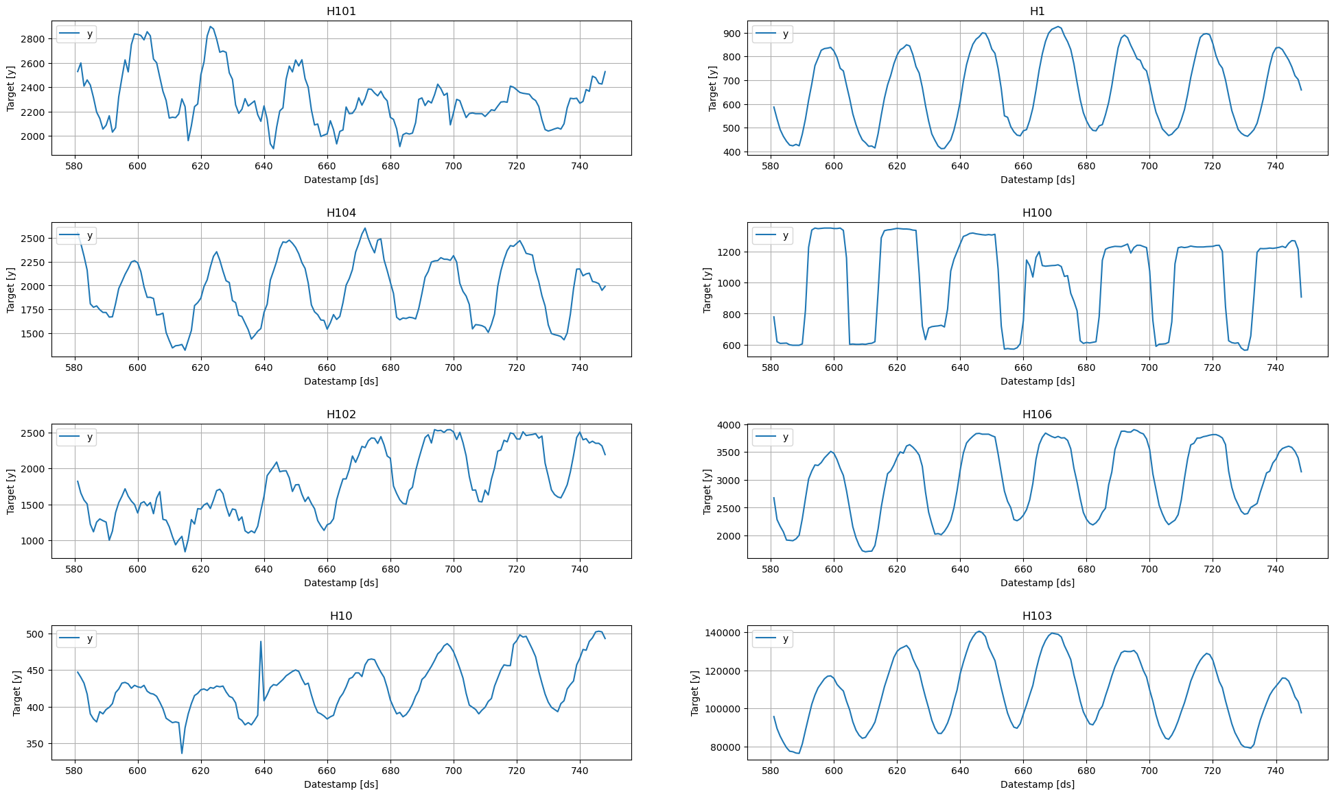
Plot some series using the plot method from the StatsForecast class. This method prints 8 random series from the dataset and is useful for basic EDA.
Note
The StatsForecast.plot method uses Plotly as a defaul engine. You can change to MatPlotLib by setting engine="matplotlib".
from statsforecast import StatsForecast
StatsForecast.plot(Y_df)
Train multiple models for many series
StatsForecast can train many models on many time series efficiently.
Start by importing and instantiating the desired models. StatsForecast offers a wide variety of models grouped in the following categories:
Auto Forecast: Automatic forecasting tools search for the best parameters and select the best possible model for a series of time series. These tools are useful for large collections of univariate time series. Includes automatic versions of: Arima, ETS, Theta, CES.
Exponential Smoothing: Uses a weighted average of all past observations where the weights decrease exponentially into the past. Suitable for data with no clear trend or seasonality. Examples: SES, Holt’s Winters, SSO.
Benchmark models: classical models for establishing baselines. Examples: Mean, Naive, Random Walk
Intermittent or Sparse models: suited for series with very few non-zero observations. Examples: CROSTON, ADIDA, IMAPA
Multiple Seasonalities: suited for signals with more than one clear seasonality. Useful for low-frequency data like electricity and logs. Examples: MSTL.
Theta Models: fit two theta lines to a deseasonalized time series, using different techniques to obtain and combine the two theta lines to produce the final forecasts. Examples: Theta, DynamicTheta
AutoARIMA: Automatically selects the best ARIMA (AutoRegressive Integrated Moving Average) model using an information criterion. Ref: AutoARIMA.
HoltWinters: triple exponential smoothing, Holt-Winters’ method is an extension of exponential smoothing for series that contain both trend and seasonality. Ref: HoltWinters
DynamicOptimizedTheta: The theta family of models has been shown to perform well in various datasets such as M3. Models the deseasonalized time series. Ref: DynamicOptimizedTheta.
Import and instantiate the models. Setting the season_length argument is sometimes tricky. This article on Seasonal periods) by the master, Rob Hyndmann, can be useful.
from statsforecast.models import ( AutoARIMA, HoltWinters, CrostonClassic as Croston, HistoricAverage, DynamicOptimizedTheta as DOT, SeasonalNaive, MSTL)
# Create a list of models and instantiation parametersmodels = [ AutoARIMA(season_length=24), HoltWinters(), Croston(), SeasonalNaive(season_length=24), HistoricAverage(), DOT(season_length=24), MSTL]
We fit the models by instantiating a new StatsForecast object with the following parameters:
models: a list of models. Select the models you want from models and import them.
n_jobs: n_jobs: int, number of jobs used in the parallel processing, use -1 for all cores.
fallback_model: a model to be used if a model fails.
Any settings are passed into the constructor. Then you call its fit method and pass in the historical data frame.
# Instantiate StatsForecast class as sfsf = StatsForecast( df=Y_df, models=models, freq='H', n_jobs=-1, fallback_model = SeasonalNaive(season_length=7))
Note
StatsForecast achieves its blazing speed using JIT compiling through Numba. The first time you call the statsforecast class, the fit method should take around 5 seconds. The second time -once Numba compiled your settings- it should take less than 0.2s.
The forecast method takes two arguments: forecasts next h (horizon) and level.
h (int): represents the forecast h steps into the future. In this case, 12 months ahead.
level (list of floats): this optional parameter is used for probabilistic forecasting. Set the level (or confidence percentile) of your prediction interval. For example, level=[90] means that the model expects the real value to be inside that interval 90% of the times.
The forecast object here is a new data frame that includes a column with the name of the model and the y hat values, as well as columns for the uncertainty intervals. Depending on your computer, this step should take around 1min. (If you want to speed things up to a couple of seconds, remove the AutoModels like ARIMA and Theta)
Note
The forecast method is compatible with distributed clusters, so it does not store any model parameters. If you want to store parameters for every model you can use the fit and predict methods. However, those methods are not defined for distrubed engines like Spark, Ray or Dask.
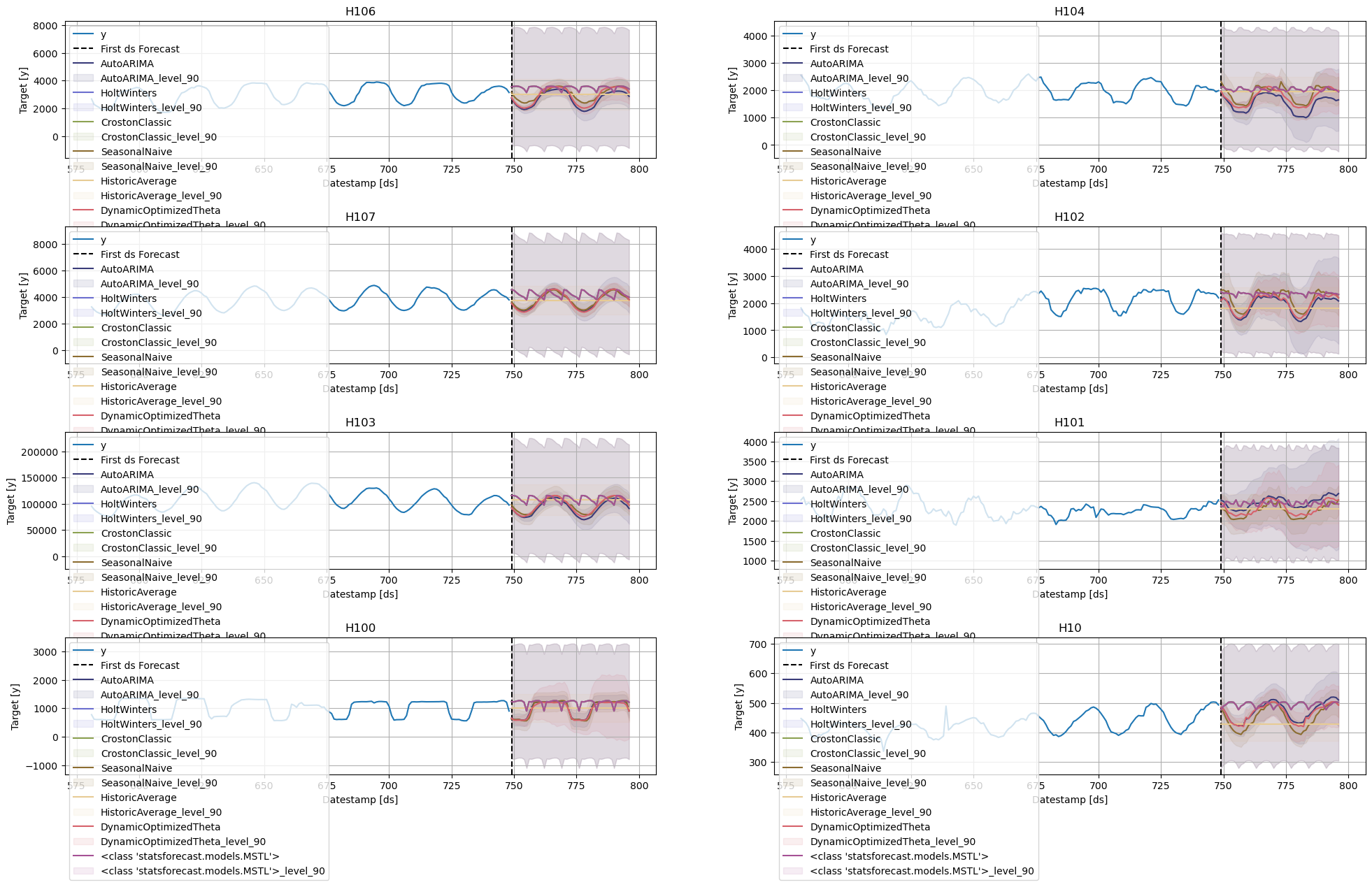
Plot the results of 8 random series using the StatsForecast.plot method.
sf.plot(Y_df,forecasts_df)
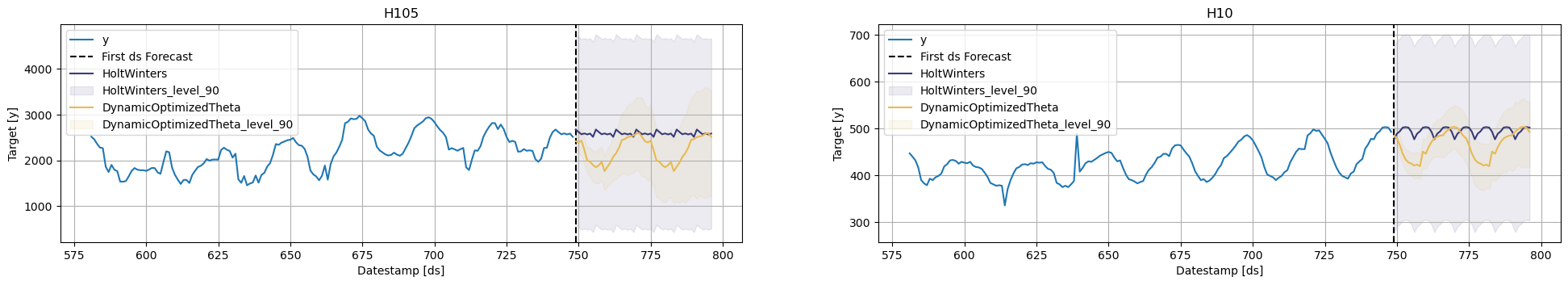
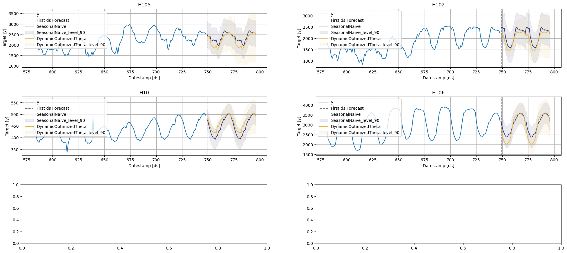
The StatsForecast.plot allows for further customization. For example, plot the results of the different models and unique ids.
# Plot to unique_ids and some selected modelssf.plot(Y_df, forecasts_df, models=["HoltWinters","DynamicOptimizedTheta"], unique_ids=["H10", "H105"], level=[90])
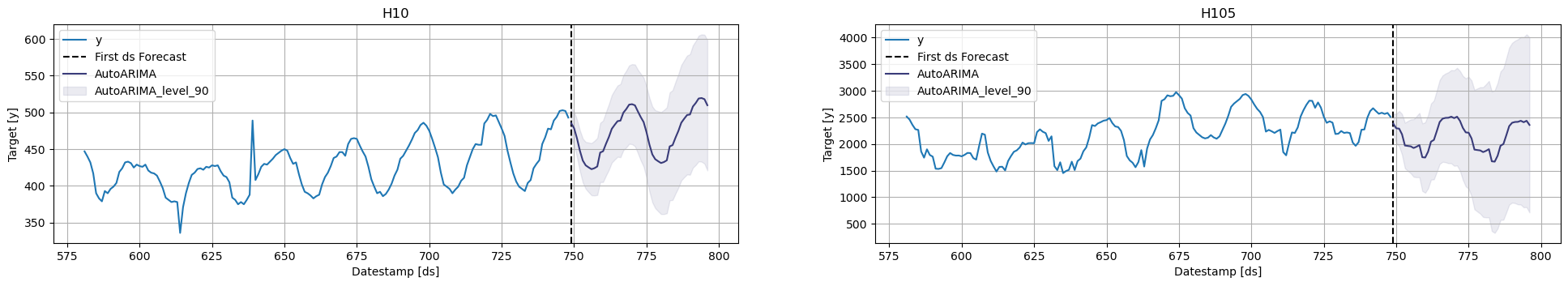
# Explore other models
sf.plot(Y_df, forecasts_df, models=["AutoARIMA"], unique_ids=["H10", "H105"], level=[90])
Evaluate the model’s performance
In previous steps, we’ve taken our historical data to predict the future. However, to asses its accuracy we would also like to know how the model would have performed in the past. To assess the accuracy and robustness of your models on your data perform Cross-Validation.
With time series data, Cross Validation is done by defining a sliding window across the historical data and predicting the period following it. This form of cross-validation allows us to arrive at a better estimation of our model’s predictive abilities across a wider range of temporal instances while also keeping the data in the training set contiguous as is required by our models.
The following graph depicts such a Cross Validation Strategy:
Cross-validation of time series models is considered a best practice but most implementations are very slow. The statsforecast library implements cross-validation as a distributed operation, making the process less time-consuming to perform. If you have big datasets you can also perform Cross Validation in a distributed cluster using Ray, Dask or Spark.
In this case, we want to evaluate the performance of each model for the last 2 days (n_windows=2), forecasting every second day (step_size=48). Depending on your computer, this step should take around 1 min.
Tip
Setting n_windows=1 mirrors a traditional train-test split with our historical data serving as the training set and the last 48 hours serving as the testing set.
The cross_validation method from the StatsForecast class takes the following arguments.
df: training data frame
h (int): represents h steps into the future that are being forecasted. In this case, 24 hours ahead.
step_size (int): step size between each window. In other words: how often do you want to run the forecasting processes.
n_windows(int): number of windows used for cross validation. In other words: what number of forecasting processes in the past do you want to evaluate.
The crossvaldation_df object is a new data frame that includes the following columns:
unique_id index: (If you dont like working with index just run forecasts_cv_df.resetindex())
ds: datestamp or temporal index
cutoff: the last datestamp or temporal index for the n_windows. If n_windows=1, then one unique cuttoff value, if n_windows=2 then two unique cutoff values.
y: true value
"model": columns with the model’s name and fitted value.
crossvaldation_df.head()
ds
cutoff
y
AutoARIMA
HoltWinters
CrostonClassic
SeasonalNaive
HistoricAverage
DynamicOptimizedTheta
<class 'statsforecast.models.MSTL'>
unique_id
H1
701
700
619.0
603.925415
847.0
742.668762
691.0
661.674988
612.767517
847.0
H1
702
700
565.0
507.591736
820.0
742.668762
618.0
661.674988
536.846252
820.0
H1
703
700
532.0
481.281677
790.0
742.668762
563.0
661.674988
497.824280
790.0
H1
704
700
495.0
444.410248
784.0
742.668762
529.0
661.674988
464.723236
784.0
H1
705
700
481.0
421.168762
752.0
742.668762
504.0
661.674988
440.972351
752.0
Next, we will evaluate the performance of every model for every series using common error metrics like Mean Absolute Error (MAE) or Mean Square Error (MSE) Define a utility function to evaluate different error metrics for the cross validation data frame.
First import the desired error metrics from mlforecast.losses. Then define a utility function that takes a cross-validation data frame as a metric and returns an evaluation data frame with the average of the error metric for every unique id and fitted model and all cutoffs.
from utilsforecast.losses import msefrom utilsforecast.evaluation import evaluate
def evaluate_cross_validation(df, metric): models = df.drop(columns=['unique_id', 'ds', 'cutoff', 'y']).columns.tolist() evals = []# Calculate loss for every unique_id and cutoff. for cutoff in df['cutoff'].unique(): eval_ = evaluate(df[df['cutoff'] == cutoff], metrics=[metric], models=models) evals.append(eval_) evals = pd.concat(evals) evals = evals.groupby('unique_id').mean(numeric_only=True) # Averages the error metrics for all cutoffs for every combination of model and unique_id evals['best_model'] = evals.idxmin(axis=1)return evals
Warning
You can also use Mean Average Percentage Error (MAPE), however for granular forecasts, MAPE values are extremely hard to judge and not useful to assess forecasting quality.
Create the data frame with the results of the evaluation of your cross-validation data frame using a Mean Squared Error metric.
Create a summary table with a model column and the number of series where that model performs best. In this case, the Arima and Seasonal Naive are the best models for 10 series and the Theta model should be used for two.
summary_df = evaluation_df.groupby('best_model').size().sort_values().to_frame()summary_df.reset_index().columns = ["Model", "Nr. of unique_ids"]
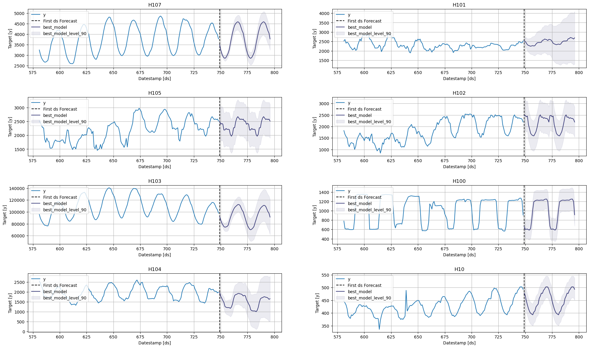
You can further explore your results by plotting the unique_ids where a specific model wins.
Define a utility function that takes your forecast’s data frame with the predictions and the evaluation data frame and returns a data frame with the best possible forecast for every unique_id.