Everything to know about image embeddings: what a good visual representation is, the mid-2026 model landscape (DINOv3 vs CLIP/SigLIP vs supervised features), how embeddings are evaluated, and runnable code that builds a real image-retrieval index.
Author
Benedict Thekkel
1. What is Image Feature Extraction?
Image feature extraction turns an image into a fixed-length vector (an embedding, typically 384-1536 floats) whose geometry is the product. Nobody consumes the vector for its own sake: the whole point is that distance in the embedding space tracks semantic similarity, so nearest neighbours of a query are pictures of the same thing.
Input. A single RGB image, resized and normalised by the model’s AutoImageProcessor (224x224 or 518x518 is typical). Nothing else - no labels, no text, no prompts.
Output. One of two things, and confusing them is the most common mistake in this task:
Output
Shape
What it is
Used for
Global embedding
[D]
one vector per image (the CLS token, or a pooled patch mean)
A ViT-B/14 at 224px gives 256 patch tokens + 1 CLS token; DINOv3 adds 4 register tokens on top of that. last_hidden_state holds all of them; the global vector is something you choose out of that tensor (section 9 - this is the single highest-leverage decision in the notebook).
Neighbouring tasks (all of them consume or produce these vectors):
Task
Relationship to embeddings
Notebook / tool
Image classification
a classifier’s penultimate layer is an embedding - the “supervised features” baseline
01_Image_Classification
Zero-shot classification
cosine similarity between an image embedding and text embeddings of class names
11_Zero_Shot_Image_Classification
Keypoint detection / matching
the classical local-feature ancestor (SIFT, ORB): many small descriptors instead of one global vector
17_Keypoint_Detection
Segmentation, depth
linear heads on top of dense patch features
03_Image_Segmentation, 00_Depth_Estimation
Text feature extraction
the exact text analogue - same metrics, same FAISS index
the infrastructure that makes embeddings usable at scale
FAISS, hnswlib, ScaNN, pgvector
2. Real-World Use Cases
Embeddings are the least visible and most widely deployed vision task: almost every “find me something like this” button in a product is a cosine similarity over a vector index.
Fine-grained similarity (this exact sneaker, not “a shoe”); index recall at billions of items
Photo library search by text
Consumer (Apple Photos, Google Photos)
“dog on a beach” -> your photos
Cross-modal (needs a language-aligned model); must run on device, private
Near-duplicate detection and copyright / CSAM matching
Content platforms (Meta PDQ, YouTube Content ID)
Uploaded image -> hash / vector match against a banned set
Robustness to crop, re-encode, watermark; precision (a false positive is a wrongful takedown)
Recommendation and cold-start ranking
Media, marketplaces
Item image -> vector feature for a ranker
Throughput (millions of items/day); embedding dimension = storage cost
Industrial anomaly detection
Manufacturing (MVTec-style inspection)
Product photo -> distance to the “normal” patch-feature distribution
Dense patch features, not just a global vector; no defect labels available
Medical / satellite retrieval
Healthcare, earth observation
Scan or tile -> similar historical cases
Severe domain shift from web images; DINOv3 ships a satellite-pretrained variant for exactly this
RAG over images / agent memory
LLM applications
Screenshot or document page -> retrieved context for a VLM
Cross-modal alignment; latency inside an agent loop
Clustering and dataset curation
ML infrastructure (LAION, DataComp, LVD-142M itself)
Billions of images -> dedup + balanced sample
Cost per image; embedding quality is dataset quality
What the ImageNet linear-probe number hides. An 87% linear probe on ImageNet tells you almost nothing about whether the model will find your duplicate. Three things break in production. (1) Domain shift: the model was trained on web photos, and X-rays, satellite tiles, CAD renders and receipts are not web photos - k-NN accuracy can collapse by 30+ points, and the fix is usually a domain-pretrained backbone rather than a better generic one. (2) The metric space is not calibrated: cosine 0.83 does not mean “duplicate” - the threshold is dataset-dependent and drifts every time you change the backbone, so every deployed system needs a re-tuned threshold and a re-embedded index (re-embedding a billion-image index is a migration, not a config change). (3) The distance you optimised is not the distance the user means: CLIP will happily rank a drawing of a golden retriever next to a photo of one, because that is what its training objective rewards; a dedup system considers that a false positive. Add the boring operational realities - embedding dimension times number of items is a hard RAM budget, and ANN search trades recall for latency at exactly the point where you stop being able to measure it.
3. How Modern Image Feature Extraction Works
The classical era (1999-2012). SIFT (1999), SURF, ORB: hand-designed local descriptors around detected keypoints, aggregated into a global vector by bag-of-visual-words / VLAD / Fisher vectors. Dead for semantics, still alive for geometry - SfM, SLAM and homography estimation still use local descriptors (see 17_Keypoint_Detection), because a global embedding cannot tell you where the match is.
Supervised features (2012-2019). Chop the head off an ImageNet CNN and use the penultimate layer. Cheap, effective, and still the right baseline - but the features are shaped by 1000 classes, so anything outside that taxonomy (textures, defects, document layouts) is represented badly.
Contrastive self-supervision (2020). SimCLR and MoCo: two augmented views of an image are positives, every other image in the batch is a negative, InfoNCE pulls and pushes. Works, but needs lots of negatives - hence SimCLR’s 4096-image batches and MoCo’s momentum queue - and false negatives (two different photos of the same breed) actively hurt.
Non-contrastive / self-distillation (2020-2021). BYOL and SimSiam showed you can drop negatives entirely: a student predicts a momentum-EMA teacher’s output for another view. The obvious failure - collapse to a constant vector - is prevented by architectural asymmetry (predictor head, stop-gradient) rather than by negatives. DINO (2021) made this a ViT recipe: EMA teacher, multi-crop, and two anti-collapse tricks that are the whole trick - centering (subtract a running mean from the teacher logits, which prevents one dimension dominating) and sharpening (a low teacher temperature, which prevents uniform output). The bonus discovery: DINO’s attention maps segment objects with no supervision at all. SwAV (2020) took a third route, contrasting cluster assignments instead of features.
Masked image modelling (2021-2022). MAE masks 75% of patches and reconstructs pixels; BEiT reconstructs discrete visual tokens. Fast to pretrain and an excellent fine-tuning initialisation, but reconstruction optimises for pixel-level detail, not for linear separability - so MAE’s linear probe and k-NN accuracy are far below DINO’s even when its fine-tuned accuracy is competitive. Section 12 reproduces this gap. If you are fine-tuning, MIM is fine; if you are embedding, it is not.
Language supervision (2021-2023). CLIP put images and text in one shared space trained by contrastive image-text matching over 400M pairs; SigLIP (2023) replaced the batch-wide softmax with a pairwise sigmoid loss, which removes the all-gather and lets you train well at small batch sizes. This bought the killer feature - search images with a text string - at a cost: the objective only needs the image vector to be closer to its caption than to other captions, and captions are coarse (“a dog”), so fine-grained purely-visual distinctions get compressed.
DINOv2 (2023). The turning point: DINO + iBOT objectives, careful data curation (LVD-142M, retrieval-deduplicated from a raw web crawl), and distillation from a ViT-g teacher into ViT-S/B/L. It was the first SSL model whose frozen, off-the-shelf features beat weakly-supervised (CLIP-family) features on most benchmarks - especially dense ones. The “registers” follow-up (2023) found that ViTs dump global information into a few high-norm background patch tokens, producing artifact-ridden attention maps, and fixed it by adding dedicated register tokens.
DINOv3 (Aug 2025). Scale it: a 7B-param ViT trained on LVD-1689M (~1.7B curated images), then distilled into a ViT-S/S+/B/L/H+ and ConvNeXt family. Its key contribution is Gram anchoring: over a long training run, dense patch features degrade (patch-to-patch similarity gets noisy) even while global features keep improving, so DINOv3 adds a loss that keeps the student’s patch Gram matrix (the matrix of pairwise patch similarities) close to that of an earlier, cleaner “Gram teacher”. The result is dense features that stay sharp at scale. Caveat: the weights are under a custom Meta “DINOv3 License” and are gated with manual approval - not Apache/MIT, so check the terms before shipping it.
The multimodal-embedding line (2024-2026). SigLIP 2 (Feb 2025) folds captioning, self-distillation and dense objectives into the SigLIP recipe and is the strongest general-purpose open image-text encoder in the base size class; Meta’s Perception Encoder (Apr 2025) showed that a well-tuned contrastive model’s intermediate layers rival DINOv2-g on spatial tasks and AIMv2 on language tasks - i.e. “the best visual embeddings are not at the output of the network”. Alongside these sit unified text+image embedders built for RAG (jina-clip-v2, nomic-embed-vision, MegaPairs/VLM2Vec-style models) that emit one vector for either modality.
Cheat sheet:
Family
Text-aligned?
Fine-grained visual
Dense/patch features
k-NN probe
Typical use
Supervised ImageNet ViT/ConvNeXt
no
ok (in-taxonomy)
weak
good
cheap baseline, in-domain classes
MAE / BEiT (MIM)
no
weak frozen
ok
poor
fine-tuning init, not embedding
CLIP / SigLIP / SigLIP 2
yes
moderate
weak-moderate
good
text-to-image search, zero-shot, RAG
DINOv2 / DINOv3 (SSL)
no
best
best
best
retrieval, dedup, dense heads, anomaly
Perception Encoder
yes
strong
strong (mid layers)
strong
when you want both, from one model
The honest summary in mid-2026: if you need text queries, you need a CLIP-family model; if you need the sharpest purely-visual geometry, you want DINOv3. Many production systems run both and concatenate.
4. Evaluation Metrics
Embeddings have no output to score directly, so every metric is a proxy task on frozen features. Two of them are standard, they measure different things, and they disagree often enough that you should always report both.
1. k-NN top-1 accuracy. Embed a labelled train set, embed a test image, take the k nearest neighbours by cosine, majority-vote the label. This measures the local metric structure - is my neighbourhood full of my own class? It is the metric that actually predicts retrieval quality, and it needs no training.
2. Linear-probe accuracy. Freeze the backbone, train a single linear layer (logistic regression) on the embeddings. This measures linear separability - is the class information present along some hyperplane? A model can be linearly separable but metrically ugly (classes separable but far from compact), which is exactly how MIM models score respectably on linear probes while collapsing on k-NN.
3. Retrieval metrics. For a query \(q\) with a relevant set \(R_q\) out of a gallery, ranked by cosine:
\[\mathrm{Recall}@k = \frac{1}{|Q|}\sum_{q \in Q} \mathbb{1}\left[\,\exists\, i \le k : \mathrm{rank}_q(i) \in R_q \right]\]
Recall@k only asks “did anything relevant land in the top k” (the right metric for “show me 5 similar products”); mAP scores the whole ranking (the right metric for the Oxford/Paris landmark benchmarks). MRR (mean reciprocal rank of the first hit) is the middle ground.
4. Alignment and uniformity (Wang and Isola, 2020) - a diagnostic, not a score. On the unit sphere, good contrastive features are aligned (positive pairs close) and uniform (features spread out, not collapsed):
Both are lower-is-better. If your fine-tune tanks, this tells you which way it broke: alignment up = the model stopped matching positives; uniformity up (toward 0) = representation collapse.
5. Cost metrics that decide the architecture. Embedding dimension (bytes per image: 768 fp32 = 3 KB, so 100M images = 300 GB of RAM before any index overhead) and throughput (images/sec). Matryoshka Representation Learning (MRL) trains the vector so that its first 64/128/256 dims are themselves usable embeddings, letting you truncate for a cheap first-pass shortlist and rerank with the full vector.
The one rule that breaks everything if you skip it: L2-normalise before you compare. Cosine similarity equals a dot product only on unit vectors, and every ANN index that advertises “inner product” search assumes you did this. Embedding norm correlates with things you do not want in your ranking (image contrast, object size), so an unnormalised dot product quietly ranks by brightness.
# The metric toolbox. Defined once here on fabricated embeddings, reused for real ones below.import torchdef l2_normalize(x, eps=1e-12):"Project rows onto the unit sphere. Do this before EVERY cosine / dot-product comparison."return x / x.norm(dim=-1, keepdim=True).clamp_min(eps)def cosine_sim(q, g):"Cosine similarity matrix [Nq, Ng] between query and gallery embeddings (raw, unnormalised)."return l2_normalize(q.float()) @ l2_normalize(g.float()).Tdef knn_top1(q, q_lab, g, g_lab, k=5):"k-NN classification accuracy: majority vote over the k nearest gallery items." sims = cosine_sim(q, g) idx = sims.topk(k, dim=1).indices # [Nq, k] votes = g_lab[idx] # [Nq, k] n_cls =int(max(g_lab.max(), q_lab.max())) +1 counts = torch.zeros(len(q), n_cls) counts.scatter_add_(1, votes, torch.ones_like(votes, dtype=torch.float))return (counts.argmax(1) == q_lab).float().mean().item()def recall_at_k(q, q_lab, g, g_lab, k=5):"Fraction of queries with at least one same-class item in the top k." idx = cosine_sim(q, g).topk(k, dim=1).indicesreturn (g_lab[idx] == q_lab[:, None]).any(1).float().mean().item()def mean_ap(q, q_lab, g, g_lab):"Mean average precision over the full ranking (the Oxford/Paris retrieval metric)." order = cosine_sim(q, g).argsort(dim=1, descending=True) rel = (g_lab[order] == q_lab[:, None]).float() # [Nq, Ng] relevance in rank order cum = rel.cumsum(1) prec_at_k = cum / torch.arange(1, rel.shape[1] +1).float() ap = (prec_at_k * rel).sum(1) / rel.sum(1).clamp_min(1)return ap.mean().item()def align_uniform(view_a, view_b, t=2.0):"Wang and Isola (2020) alignment (positive-pair distance) and uniformity (log-MMD to a Gaussian kernel)." a, b = l2_normalize(view_a.float()), l2_normalize(view_b.float()) alignment = (a - b).norm(dim=1).pow(2).mean().item() sq = torch.pdist(a, p=2).pow(2) uniformity = sq.mul(-t).exp().mean().log().item()return alignment, uniformity# --- toy check on fabricated embeddings: 3 classes, 3 gaussian blobs in 8-D -------------torch.manual_seed(0)centers = torch.randn(3, 8) *3g_lab = torch.arange(3).repeat_interleave(20) # 60 gallery itemsgallery = centers[g_lab] + torch.randn(60, 8) *0.7q_lab = torch.arange(3).repeat_interleave(4) # 12 queriesqueries = centers[q_lab] + torch.randn(12, 8) *0.7print("k-NN top-1 :", round(knn_top1(queries, q_lab, gallery, g_lab, k=5), 3))print("Recall@5 :", round(recall_at_k(queries, q_lab, gallery, g_lab, k=5), 3))print("mAP :", round(mean_ap(queries, q_lab, gallery, g_lab), 3))# Cosine == dot product ONLY on unit vectors. Scaling one row by 10 leaves cosine# untouched but multiplies the raw dot product by 10 - i.e. an unnormalised index# ranks by vector norm, which is a property of the image, not of its content.a, b = gallery[0], gallery[1] *10.0print("raw dot :", round(float(a @ b), 3))print("cosine :", round(float(cosine_sim(a[None], b[None])[0, 0]), 3))print("dot after L2 norm:", round(float(l2_normalize(a[None]) @ l2_normalize(b[None]).T), 3))# Alignment/uniformity: treat a lightly-jittered copy as the positive view.print("align, uniform :", [round(v, 3) for v in align_uniform(gallery, gallery + torch.randn(60, 8) *0.2)])
Embedding models are trained on huge uncurated (or carefully de-duplicated) web crawls and evaluated on small labelled probes. The two sets barely overlap.
We evaluate on Oxford-IIIT Pet (timm/oxford-iiit-pet): 37 breeds, ungated, parquet-backed, and fine-grained - which is exactly the axis where DINOv2/DINOv3 pull away from CLIP. It fits the box: we sub-sample ~320 images. ImageNet-1k is gated (you must accept terms on the Hub) and is far too big to probe on this machine anyway.
6. The Model Landscape (mid-2026)
The authoritative rankings are MIEB (130 image / image-text tasks, 38 languages, folded into the MTEB leaderboard) and MMEB (36 datasets, instruction-following multimodal embedders). MIEB’s headline finding is worth internalising: no single model wins all eight task categories - the model that tops linear probing is not the model that tops interleaved retrieval or document understanding.
Model
Params
License
Scope
Architecture
Best for
DINOv3 ViT-7B/16
6.7B
DINOv3 License (gated)
vision only
SSL + Gram anchoring
SOTA dense + global features. Way past 12 GB - use a distilled child
DINOv3 ViT-B/16
86M, D=768
DINOv3 License (gated)
vision only
distilled from the 7B
best runnable visual embedder; needs manual Hub approval
DINOv3 ViT-L/16
303M, D=1024
DINOv3 License (gated)
vision only
distilled
fits 12 GB; the quality/size sweet spot
DINOv3 ConvNeXt-B
89M
DINOv3 License
vision only
ConvNeXt
edge / ONNX / non-ViT stacks
DINOv3 ViT-L/16 SAT-493M
303M
DINOv3 License
satellite
distilled
earth observation (huge domain-shift win)
DINOv2 ViT-B/14
86M, D=768
Apache 2.0
vision only
DINO + iBOT
the ungated default; what to reach for first
DINOv2 ViT-L/14 + registers
304M
Apache 2.0
vision only
+ register tokens
clean attention maps, dense heads
SigLIP 2 base/16
375M total, D=768
Apache 2.0
image + text, multilingual
sigmoid ITC + captioning
best open language-aligned base model
CLIP ViT-B/32
151M, D=512
MIT
image + text
softmax ITC
the ecosystem baseline; fastest text-to-image demo
Perception Encoder Core B/16
~86M vision
Apache 2.0
image + text
contrastive, mid-layer features
one model for both language and spatial tasks
AIMv2-L/14
309M
apple-amlr (restricted)
image + text
autoregressive multimodal
strong VLM backbone
jina-clip-v2
865M
CC-BY-NC-4.0 (no commercial use)
89 languages + image
dual encoder, Matryoshka dims
multilingual text+image RAG
nomic-embed-vision-v1.5
93M, D=768
Apache 2.0
image, aligned to nomic-embed-text
ViT aligned post-hoc
one index shared with a text embedder
ViT-B/16 (ImageNet-1k supervised)
86M, D=768
Apache 2.0
vision only
supervised
the honest baseline everyone forgets
ViT-MAE base
112M, D=768
Apache 2.0
vision only
masked autoencoder
a fine-tuning init, not an embedder
Who wins what. Accuracy on purely-visual similarity: DINOv3 (then DINOv2). Anything involving text: SigLIP 2 (then Perception Encoder, then CLIP). Speed and storage: CLIP ViT-B/32 - 512-d vectors and 32x32 patches make it ~4x cheaper per image than a /14 or /16 model, which is why it survives in production long after being beaten on accuracy. Tie this back to section 2: a photo-library text search must be CLIP-family (there is no other way to type a query); a dedup or defect-inspection system should be DINOv3, because it never needs text and cares only about fine-grained visual geometry.
Licensing is a real constraint here. DINOv3 is not open source - it is a custom Meta license behind a manually-approved gate. jina-clip-v2 is non-commercial. AIMv2 is under Apple’s restricted ASCL. If you need a permissive licence and good visual features, DINOv2 (Apache 2.0) remains the answer, and that is why it is this notebook’s primary model.
7. Setup
Every model loads through Hugging Face transformers - no vendor packages. Package roles:
transformers (>=5.13) + torch - all backbones (AutoModel + AutoImageProcessor, plus the image-feature-extraction pipeline)
datasets - the Oxford-IIIT Pet eval split (parquet, no loading script)
accelerate - device placement
pillow - decoding and displaying retrieved images
pyecharts - all charts
pandas - the benchmark table
numpy - PCA via SVD (no scikit-learn needed)
Deliberately not used: faiss. Exact cosine search over a few hundred vectors is one matmul, and writing it out makes the mechanics visible. At scale you swap that matmul for FAISS / hnswlib / ScaNN / pgvector - see section 16.
All downloads (sample image, HF model + dataset cache) land in DL_tasks/datasets/, which is gitignored.
# Everything runs through Hugging Face transformers - no model-specific packages.# %pip install -q torch transformers datasets accelerate pillow pyecharts pandas numpy# DINOv3 is a GATED repo (custom Meta license, manual approval). To run section 13:# 1. accept the terms at https://huggingface.co/facebook/dinov3-vitb16-pretrain-lvd1689m# 2. wait for approval, then put HF_TOKEN=hf_... in Knowledge/.env# Every other model in this notebook is ungated.
import ctypesimport ctypes.utilimport gcimport timeimport urllib.requestfrom pathlib import Pathimport torchfrom dotenv import find_dotenv, load_dotenv# Knowledge/.env sets HF_TOKEN - authenticated HF Hub requests get higher rate limits# (and are required for the gated DINOv3 weights in section 13).load_dotenv(find_dotenv(usecwd=True))device ="cuda:0"if torch.cuda.is_available() else"cpu"dtype = torch.float16 if device !="cpu"else torch.float32if device !="cpu":print(torch.cuda.get_device_name(0))print("device:", device, "| dtype:", dtype)def vram(tag=""):"Report current GPU memory (allocated / reserved). No-op on CPU."if torch.cuda.is_available(): alloc = torch.cuda.memory_allocated() /1e9 reserved = torch.cuda.memory_reserved() /1e9print(f"VRAM {tag:20s}{alloc:5.2f} GB allocated / {reserved:5.2f} GB reserved")def free_memory():"Collect garbage, empty the CUDA cache, and return freed CPU RAM to the OS." gc.collect()if torch.cuda.is_available(): torch.cuda.empty_cache() torch.cuda.ipc_collect()# glibc keeps freed CPU allocations in its arenas instead of returning them# to the OS, so RSS compounds across model sections (cpu-offloaded weights# live in system RAM). malloc_trim(0) hands the freed arenas back. See# dl-visualization-and-memory.instructions.md - not optional on a 12 GB box.try: ctypes.CDLL(ctypes.util.find_library("c") or"libc.so.6").malloc_trim(0)exceptException:pass# All downloads go to DL_tasks/datasets/ (gitignored)DATA_DIR = Path("../../datasets")DATA_DIR.mkdir(exist_ok=True)HF_CACHE =str(DATA_DIR /"hf_cache")# The canonical COCO two-cats image - our single-image sanity checkSAMPLE = DATA_DIR /"cats.jpg"ifnot SAMPLE.exists(): urllib.request.urlretrieve("http://images.cocodataset.org/val2017/000000039769.jpg", SAMPLE )
from datasets import load_datasetfrom PIL import Image# Oxford-IIIT Pet: 37 fine-grained cat/dog breeds, ungated, parquet-backed.# We take 8 breeds x 40 images = 320 images so the whole notebook stays inside# a few hundred MB of RAM and a couple of minutes of GPU time.N_CLASSES, PER_CLASS =8, 40pets = load_dataset("timm/oxford-iiit-pet", split="test", cache_dir=HF_CACHE)CLASS_NAMES = pets.features["label"].namesby_class = {c: [] for c inrange(N_CLASSES)}for i, lab inenumerate(pets["label"]):if lab < N_CLASSES andlen(by_class[lab]) < PER_CLASS: by_class[lab].append(i)assertall(len(v) == PER_CLASS for v in by_class.values()), "not enough images per class"keep = [i for c inrange(N_CLASSES) for i in by_class[c]] # grouped by class, in class ordersubset = pets.select(keep)# Materialise 320 small PIL images once (RGB, <=512px) and free the Arrow handles.IMAGES = [im.convert("RGB") for im in subset["image"]]LABELS = torch.tensor(subset["label"])LABEL_NAMES = [CLASS_NAMES[i] for i inrange(N_CLASSES)]# Gallery / query split: 25 per class indexed, 15 per class queried.is_query = torch.cat([torch.arange(PER_CLASS) >=25for _ inrange(N_CLASSES)])G_IDX = (~is_query).nonzero().squeeze(1) # 200 gallery imagesQ_IDX = is_query.nonzero().squeeze(1) # 120 query imagesG_LAB, Q_LAB = LABELS[G_IDX], LABELS[Q_IDX]print(f"{len(IMAGES)} images | {N_CLASSES} breeds: {', '.join(LABEL_NAMES)}")print(f"gallery {len(G_IDX)} | queries {len(Q_IDX)}")del pets, subsetfree_memory()def show_row(images, size=140, captions=None):"Paste PIL images side by side into one strip (ECharts cannot draw images; PIL can)." thumbs = [im.resize((size, size)) for im in images] strip = Image.new("RGB", (size *len(thumbs), size), "white")for i, t inenumerate(thumbs): strip.paste(t, (i * size, 0))if captions:print(" | ".join(captions))return stripshow_row([IMAGES[i * PER_CLASS] for i inrange(N_CLASSES)], captions=LABEL_NAMES)
# The two workhorses used by every section below: a batched embedding driver and# a torch linear probe (no scikit-learn dependency).from IPython.display import display@torch.inference_mode()def embed_all(encode, images, batch_size=16):"""Run `encode(list_of_PIL) -> [B, D]` over all images in batches. Returns a float32 CPU tensor [N, D] plus images/sec. Everything is moved off the GPU immediately so VRAM does not grow with N. """ chunks = [] t0 = time.perf_counter()for i inrange(0, len(images), batch_size): chunks.append(encode(images[i:i + batch_size]).float().cpu()) elapsed = time.perf_counter() - t0return torch.cat(chunks), len(images) / elapseddef linear_probe(g, g_lab, q, q_lab, epochs=300, lr=0.05, wd=1e-4):"Train a logistic regression on frozen (L2-normalised) features; return test accuracy." xtr, xte = l2_normalize(g.float()), l2_normalize(q.float()) clf = torch.nn.Linear(xtr.shape[1], int(g_lab.max()) +1) opt = torch.optim.AdamW(clf.parameters(), lr=lr, weight_decay=wd)for _ inrange(epochs): # full batch: 200 x 768 is tiny opt.zero_grad() torch.nn.functional.cross_entropy(clf(xtr), g_lab).backward() opt.step()with torch.inference_mode():return (clf(xte).argmax(1) == q_lab).float().mean().item()def score(emb, tag):"k-NN top-1 + Recall@5 + mAP + linear probe for one embedding matrix." g, q = emb[G_IDX], emb[Q_IDX] row =dict( dim=emb.shape[1], knn=knn_top1(q, Q_LAB, g, G_LAB, k=5), recall5=recall_at_k(q, Q_LAB, g, G_LAB, k=5),map=mean_ap(q, Q_LAB, g, G_LAB), probe=linear_probe(g, G_LAB, q, Q_LAB), )print(f"{tag:26s} d={row['dim']:4d} kNN {row['knn']:.3f} R@5 {row['recall5']:.3f} "f"mAP {row['map']:.3f} probe {row['probe']:.3f}")return row
8. DINOv2 (self-supervised visual features)
facebook/dinov2-base - 86M params, ViT-B/14, Apache 2.0, ungated. Self-distillation (DINO) plus a masked-patch objective (iBOT) on the curated LVD-142M crawl, distilled from a ViT-g teacher. Pick it when you want the best purely visual similarity you can get under a permissive licence and without a Hub approval queue.
It is a plain AutoModel, so it returns a BaseModelOutputWithPooling:
last_hidden_state -> [B, 1 + 256, 768] at 224px: CLS token first, then 256 patch tokens (14x14 patches on a 224px image gives 16x16 = 256 patches).
pooler_output -> [B, 768]. For DINOv2 this is just layernorm(last_hidden_state[:, 0]), i.e. the CLS token - there is no learned pooling head. (That is not true of every ViT - see the warning in section 12.)
The image-feature-extraction pipeline wraps this in one line, but it hides the pooling choice, which is exactly the thing you need to control. Use it for a quick look; use AutoModel for anything real.
from transformers import AutoImageProcessor, AutoModel, pipelineDINOV2 ="facebook/dinov2-base"dino_proc = AutoImageProcessor.from_pretrained(DINOV2, cache_dir=HF_CACHE)dino = AutoModel.from_pretrained(DINOV2, dtype=dtype, cache_dir=HF_CACHE).to(device).eval()vram("dinov2-base loaded")# One image, to see the raw token tensor.with torch.inference_mode(): inp = dino_proc(images=Image.open(SAMPLE), return_tensors="pt").to(device, dtype) out = dino(**inp)print("last_hidden_state:", tuple(out.last_hidden_state.shape), " (1 CLS + 256 patch tokens)")print("pooler_output :", tuple(out.pooler_output.shape))print("pooler == CLS :", torch.allclose(out.pooler_output, out.last_hidden_state[:, 0]))# The four candidate global vectors. n_prefix = number of non-patch tokens at the# front of the sequence: 1 (CLS) for DINOv2, 5 (CLS + 4 registers) for DINOv3.def vit_encode(model, proc, n_prefix=1, pooling="cls"):def encode(batch): inp = proc(images=batch, return_tensors="pt").to(device, dtype) h = model(**inp).last_hidden_state cls, patches = h[:, 0], h[:, n_prefix:]return {"cls": cls,"patch_mean": patches.mean(1),"cls+patch_mean": torch.cat([cls, patches.mean(1)], dim=-1), # the official DINOv2 probe input }[pooling]return encodet0 = time.perf_counter()DINO_EMB = {p: embed_all(vit_encode(dino, dino_proc, 1, p), IMAGES)[0]for p in ["cls", "patch_mean", "cls+patch_mean"]}print(f"embedded {len(IMAGES)} images x 3 poolings in {time.perf_counter() - t0:.1f}s")print({k: tuple(v.shape) for k, v in DINO_EMB.items()})# The one-liner equivalent (pool=True returns pooler_output, i.e. the CLS token):# pipe = pipeline("image-feature-extraction", model=DINOV2, device=device)# pipe(str(SAMPLE), pool=True, return_tensors="pt").shape -> [1, 768]del dino, dino_proc, out, inpfree_memory()vram("after dinov2")
This is the decision that most often separates a retrieval system that works from one that does not, and it is almost never discussed. last_hidden_state is [B, T, D]; you must collapse T into a single vector, and the options are not equivalent:
Choice
What it encodes
Notes
pooler_output
whatever the checkpoint’s pooling head does
Read the source. DINOv2: the CLS token. ViT-in1k: a randomly initialised dense+tanh head, because the classification checkpoint never trained one (section 12). CLIP/SigLIP: you should call get_image_features() instead, which applies the learned projection into the shared text space.
CLS token
the global summary the training objective optimised
The intended global descriptor for DINO-family models.
mean of patch tokens
the average of local content
Often better for retrieval and for texture/part-level similarity; much less sensitive to what the object-centric CLS decided was “the subject”.
concat(CLS, patch mean)
both
Doubles D (768 -> 1536). This is what Dinov2ForImageClassification actually feeds its linear layer, and what the DINOv2 paper uses for linear evaluation. Best accuracy, 2x the storage.
Then, whichever you pick: L2-normalise. Then cosine == dot product, and an inner-product ANN index gives you cosine search for free.
The cell below builds an index with each pooling choice and scores it. The numbers move by several points on the same frozen model - the pooling choice is worth as much as a model upgrade.
from pyecharts import options as optsfrom pyecharts.charts import Barpool_rows = {p: score(emb, f"dinov2 {p}") for p, emb in DINO_EMB.items()}# The vectors are unnormalised on purpose: show what skipping L2-norm costs._g, _q = DINO_EMB["cls"][G_IDX], DINO_EMB["cls"][Q_IDX]raw_dot_idx = (_q.float() @ _g.float().T).argmax(1) # rank by raw dot productcos_idx = cosine_sim(_q, _g).argmax(1) # rank by cosineprint("\nnearest-neighbour top-1 accuracy, dinov2 CLS:")print(" raw dot product :", round((G_LAB[raw_dot_idx] == Q_LAB).float().mean().item(), 3))print(" cosine (L2-norm):", round((G_LAB[cos_idx] == Q_LAB).float().mean().item(), 3))print(" disagreements :", int((raw_dot_idx != cos_idx).sum()), "/", len(Q_IDX), "queries")pools =list(pool_rows)bar = ( Bar() .add_xaxis(pools) .add_yaxis("k-NN top-1", [round(pool_rows[p]["knn"], 3) for p in pools]) .add_yaxis("Recall@5", [round(pool_rows[p]["recall5"], 3) for p in pools]) .add_yaxis("linear probe", [round(pool_rows[p]["probe"], 3) for p in pools]) .set_global_opts( title_opts=opts.TitleOpts(title="DINOv2-base: the pooling choice is worth points", subtitle="Oxford-IIIT Pet, 8 breeds, 200 gallery / 120 query"), xaxis_opts=opts.AxisOpts(name="pooled vector"), yaxis_opts=opts.AxisOpts(name="accuracy", min_=0, max_=1), tooltip_opts=opts.TooltipOpts(trigger="axis"), ))bar.render_notebook()
# The retrieval demo: exact cosine search over the 200-image gallery, then look at# what actually comes back. `sims @ ...` IS the index - at this size, one matmul.EMB = l2_normalize(DINO_EMB["cls+patch_mean"]) # best pooling from the cell abovegallery_emb, query_emb = EMB[G_IDX], EMB[Q_IDX]def retrieve(qi, k=5):"Top-k gallery neighbours of query image qi (an index into Q_IDX)." sims = query_emb[qi] @ gallery_emb.T # cosine, because both sides are unit-norm top = sims.topk(k)return top.indices, top.valuesfor qi in [0, 60, 110]: # one query from three different breeds idx, vals = retrieve(qi, k=5) q_img = IMAGES[Q_IDX[qi]] hits = [IMAGES[G_IDX[j]] for j in idx] caps = [f"{LABEL_NAMES[G_LAB[j]]}{v:.3f}"for j, v inzip(idx, vals)]print(f"\nQUERY: {LABEL_NAMES[Q_LAB[qi]]} -> top-5 by cosine") display(show_row([q_img] + hits, captions=["QUERY"] + caps))# At 200 vectors this matmul is free. At 200M vectors you swap it for an ANN index# (FAISS IndexFlatIP / IVF-PQ, hnswlib, ScaNN, or pgvector) - all of which do inner# product, i.e. they assume you L2-normalised. The rest of the code is identical.
openai/clip-vit-base-patch32 - 151M params, D=512, MIT. Two encoders trained so that an image and its caption land at the same point on a shared unit sphere. That single property buys the thing DINOv2 physically cannot do: type a sentence, get images back.
The API differs from a plain ViT:
model.get_image_features(**image_inputs) -> [B, 512] (CLS token through the learned visual projection)
Do not use vision_model(...).pooler_output for retrieval - that is the pre-projection 768-d vector and it does not live in the text space.
The price: the contrastive caption objective only has to separate an image from other captions in the batch, and captions are coarse. So CLIP is excellent at “a dog”, mediocre at “which of these 8 breeds”, and it happily rates a drawing of a golden retriever as very similar to a photo of one. Watch its fine-grained k-NN score against DINOv2’s below.
from transformers import CLIPModel, CLIPProcessorCLIP_ID ="openai/clip-vit-base-patch32"clip_proc = CLIPProcessor.from_pretrained(CLIP_ID, cache_dir=HF_CACHE)clip = CLIPModel.from_pretrained(CLIP_ID, dtype=dtype, cache_dir=HF_CACHE).to(device).eval()vram("clip loaded")def clip_encode(batch): inp = clip_proc(images=batch, return_tensors="pt").to(device, dtype)return clip.get_image_features(**inp).pooler_output # [B, 512], projected into the shared spaceCLIP_EMB, clip_ips = embed_all(clip_encode, IMAGES)print(f"{clip_ips:.1f} img/s")clip_row = score(CLIP_EMB, "clip-vit-base-patch32")# --- text -> image search: encode a SENTENCE into the SAME 512-d space ------------queries = ["a photo of a fluffy white dog","a close-up photo of a siamese cat","a photo of a small brown puppy on grass",]with torch.inference_mode(): tin = clip_proc(text=queries, return_tensors="pt", padding=True).to(device) tfeat = clip.get_text_features(**tin).pooler_output.float().cpu()sims = l2_normalize(tfeat) @ l2_normalize(CLIP_EMB).T # [3 texts, 320 images]for qi, text inenumerate(queries): top = sims[qi].topk(4)print(f'\n"{text}"') display(show_row([IMAGES[j] for j in top.indices], captions=[f"{LABEL_NAMES[LABELS[j]]}{v:.3f}"for j, v inzip(top.indices, top.values)]))# DINOv2 CANNOT do the cell above. It has no text encoder and no shared space - its# vectors are not comparable to anything but other DINOv2 vectors. That is the whole# trade-off from the section-3 table, in one cell.del clip, clip_proc, tin, tfeatfree_memory()vram("after clip")
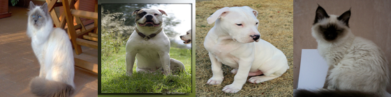
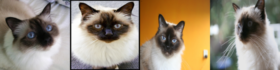
"a close-up photo of a siamese cat"
birman 0.337 | birman 0.334 | birman 0.332 | birman 0.331
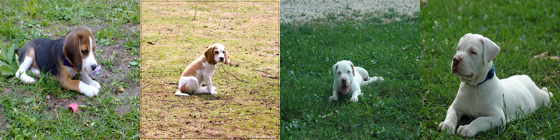
"a photo of a small brown puppy on grass"
beagle 0.312 | beagle 0.309 | american_bulldog 0.303 | american_bulldog 0.299
VRAM after clip 0.01 GB allocated / 0.02 GB reserved
11. SigLIP 2 (the stronger language-aligned option)
google/siglip2-base-patch16-224 - 375M params (vision + text towers), D=768, Apache 2.0. SigLIP swaps CLIP’s batch-wide softmax for a pairwise sigmoid loss: every image-text pair is an independent binary decision, so there is no all-gather over the batch and training works at small batch sizes. SigLIP 2 (Feb 2025) adds captioning, self-distillation and dense-prediction objectives on top, and is the best open image-text encoder in this size class. Same API as CLIP (get_image_features / get_text_features).
Two things bite people here.
The text processor needs padding="max_length". SigLIP was trained with a fixed 64-token text sequence; padding=True (pad-to-longest, the CLIP habit) silently changes the text embedding and produces garbage rankings. This is the single most reported “SigLIP is broken” bug.
Raw cosine similarities look tiny (~0.1 for a correct match, where CLIP would say ~0.3). That is the sigmoid loss’s learned logit_scale and logit_bias doing their job - the calibrated probability comes from logits_per_image. For ranking it does not matter (cosine is monotone in the logit), but do not port a CLIP similarity threshold across.
from transformers import AutoProcessorSIGLIP_ID ="google/siglip2-base-patch16-224"sig_proc = AutoProcessor.from_pretrained(SIGLIP_ID, cache_dir=HF_CACHE)siglip = AutoModel.from_pretrained(SIGLIP_ID, dtype=dtype, cache_dir=HF_CACHE).to(device).eval()vram("siglip2 loaded")def siglip_encode(batch): inp = sig_proc(images=batch, return_tensors="pt").to(device, dtype)return siglip.get_image_features(**inp).pooler_output # [B, 768]SIGLIP_EMB, sig_ips = embed_all(siglip_encode, IMAGES)print(f"{sig_ips:.1f} img/s")siglip_row = score(SIGLIP_EMB, "siglip2-base-patch16")with torch.inference_mode(): tin = sig_proc( text=["a photo of a siamese cat", "a photo of a beagle"], padding="max_length", # REQUIRED - see the note above return_tensors="pt", ).to(device) tfeat = siglip.get_text_features(**tin).pooler_output.float().cpu()sims = l2_normalize(tfeat) @ l2_normalize(SIGLIP_EMB).Tprint("\nraw cosine of the best match:", round(float(sims.max()), 3)," <- small by construction (sigmoid loss), still perfectly rankable")for qi, text inenumerate(["a photo of a siamese cat", "a photo of a beagle"]): top = sims[qi].topk(4)print(f'\n"{text}"') display(show_row([IMAGES[j] for j in top.indices], captions=[LABEL_NAMES[LABELS[j]] for j in top.indices]))del siglip, sig_proc, tin, tfeatfree_memory()vram("after siglip2")
[transformers] Model config: bos_token_id must be `None` or an integer within the vocabulary (between 0 and 31999), got 49406. This may result in unexpected behavior.
[transformers] Model config: eos_token_id must be `None` or an integer within the vocabulary (between 0 and 31999), got 49407. This may result in unexpected behavior.
VRAM siglip2 loaded        0.78 GB allocated /  0.79 GB reserved
150.7 img/s
siglip2-base-patch16       d= 768  kNN 0.925  R@5 0.983  mAP 0.754  probe 0.967

raw cosine of the best match: 0.158   <- small by construction (sigmoid loss), still perfectly rankable

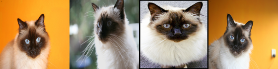
"a photo of a siamese cat"
birman | birman | birman | birman
"a photo of a beagle"
beagle | beagle | beagle | beagle
VRAM after siglip2 0.01 GB allocated / 0.02 GB reserved
12. The baselines everyone forgets: supervised ViT and MAE
Two reference points that make the DINOv2/SigLIP numbers mean something.
Supervised ImageNet features (google/vit-base-patch16-224, 86M, Apache 2.0). Load the classification checkpoint with AutoModel and you get the backbone whose penultimate layer fed the 1000-way head. These features are genuinely decent - and biased toward the ImageNet taxonomy, which happens to contain several of our dog breeds, so this baseline is flattered by the pets dataset. Footgun:ViTModel builds a pooler by default, but the classification checkpoint never trained one, so pooler_output here is a randomly initialised dense+tanh layer. Transformers warns you (newly initialized: ['pooler...']) and everyone ignores it. Take last_hidden_state[:, 0].
MAE (facebook/vit-mae-base, 112M, Apache 2.0). The masked-autoencoder that reconstructs 75% masked pixels. Excellent when fine-tuned; poor when frozen, because pixel reconstruction never asks for linear separability. Footgun:ViTMAEModel randomly masks 75% of patches at inference too - config.mask_ratio defaults to 0.75, so your embeddings are computed from a quarter of the image and change on every call. Pass mask_ratio=0.0. Even after fixing that, watch the k-NN score fall off a cliff while the linear probe holds up better: that is the MIM signature, and it is exactly why “good features” needs two metrics.
# --- supervised ImageNet-1k ViT ---------------------------------------------------SUP_ID ="google/vit-base-patch16-224"sup_proc = AutoImageProcessor.from_pretrained(SUP_ID, cache_dir=HF_CACHE)sup = AutoModel.from_pretrained(SUP_ID, dtype=dtype, cache_dir=HF_CACHE).to(device).eval()# NOTE: sup.pooler is randomly initialised (the in1k checkpoint has no pooler).# Use the CLS token from last_hidden_state, never pooler_output, for this checkpoint.SUP_EMB, sup_ips = embed_all(vit_encode(sup, sup_proc, 1, "cls"), IMAGES)sup_row = score(SUP_EMB, "vit-b/16 supervised")del sup, sup_procfree_memory()# --- MAE (masked image modelling) -------------------------------------------------MAE_ID ="facebook/vit-mae-base"mae_proc = AutoImageProcessor.from_pretrained(MAE_ID, cache_dir=HF_CACHE)mae = AutoModel.from_pretrained( MAE_ID, dtype=dtype, cache_dir=HF_CACHE, mask_ratio=0.0, # CRITICAL: default 0.75 masks 3/4 of the patches at inference).to(device).eval()MAE_EMB, mae_ips = embed_all(vit_encode(mae, mae_proc, 1, "cls"), IMAGES)mae_row = score(MAE_EMB, "vit-mae-base (frozen)")del mae, mae_procfree_memory()vram("after baselines")print("\nThe MIM signature: MAE's linear probe stays respectable while its k-NN collapses.")print("Linear separability (probe) and local metric structure (k-NN) are NOT the same thing,")print("and retrieval only cares about the second one.")
[transformers] ViTModel LOAD REPORT from: google/vit-base-patch16-224

Key                 | Status     |

--------------------+------------+-

classifier.weight   | UNEXPECTED |

classifier.bias     | UNEXPECTED |

pooler.dense.bias   | MISSING    |

pooler.dense.weight | MISSING    |


Notes:

- UNEXPECTED:   can be ignored when loading from different task/architecture; not ok if you expect identical arch.

- MISSING:  those params were newly initialized because missing from the checkpoint. Consider training on your downstream task.
vit-mae-base (frozen)      d= 768  kNN 0.433  R@5 0.775  mAP 0.233  probe 0.733
VRAM after baselines       0.01 GB allocated /  0.02 GB reserved

The MIM signature: MAE's linear probe stays respectable while its k-NN collapses.
Linear separability (probe) and local metric structure (k-NN) are NOT the same thing,
and retrieval only cares about the second one.
13. DINOv3 (the current visual-feature leader)
facebook/dinov3-vitb16-pretrain-lvd1689m - 86M params, D=768, distilled from the 7B teacher trained on LVD-1689M (~1.7B curated images). The headline idea is Gram anchoring: patch-level features quietly rot over a long training run, so DINOv3 regularises the student’s patch-to-patch Gram matrix toward an earlier, cleaner teacher. It is the strongest off-the-shelf frozen visual backbone available, and its dense features are in a different class from DINOv2’s.
Two practical differences from DINOv2:
Sequence layout.last_hidden_state is [B, 1 + 4 + 196, 768] at 224px: CLS, then 4 register tokens, then 196 patch tokens (16x16 patches). Slice patches from index 5, not 1 - n_prefix=5 in our helper. Getting this wrong silently mixes register tokens into your patch mean.
License and gating. The weights are under a custom Meta “DINOv3 License”, not Apache/MIT, and the repo is gated with manual approval - you accept the terms on the Hub, wait, then authenticate with HF_TOKEN. Read the license before shipping it commercially; that restriction is the single best reason to stay on DINOv2.
The cell is guarded, so it skips cleanly if you have not been granted access.
DINOV3_ID ="facebook/dinov3-vitb16-pretrain-lvd1689m"# gated: accept terms + manual approvalDINOV3_EMB, dinov3_row, dinov3_ips =None, None, Nonetry: d3_proc = AutoImageProcessor.from_pretrained(DINOV3_ID, cache_dir=HF_CACHE) d3 = AutoModel.from_pretrained(DINOV3_ID, dtype=dtype, cache_dir=HF_CACHE).to(device).eval() vram("dinov3 loaded")with torch.inference_mode(): inp = d3_proc(images=Image.open(SAMPLE), return_tensors="pt").to(device, dtype) h = d3(**inp).last_hidden_stateprint("last_hidden_state:", tuple(h.shape), " (1 CLS + 4 registers + 196 patches)")# n_prefix=5: skip CLS AND the 4 register tokens when mean-pooling patches. DINOV3_EMB, dinov3_ips = embed_all(vit_encode(d3, d3_proc, 5, "cls+patch_mean"), IMAGES) dinov3_row = score(DINOV3_EMB, "dinov3-vitb16")print(f"{dinov3_ips:.1f} img/s")del d3, d3_proc, h, inp free_memory() vram("after dinov3")exceptExceptionas e: # GatedRepoError / 401 if not approved, or no HF_TOKENprint(f"DINOv3 unavailable, skipping: {type(e).__name__}: {e}")print("Accept the license at https://huggingface.co/facebook/dinov3-vitb16-pretrain-lvd1689m")print("and set HF_TOKEN in Knowledge/.env once approved.") free_memory()
DINOv3 unavailable, skipping: OSError: You are trying to access a gated repo.
Make sure to have access to it at https://huggingface.co/facebook/dinov3-vitb16-pretrain-lvd1689m.
403 Client Error. (Request ID: Root=1-6a62efa2-0903d77b7fb252e55d529f91;5fa01410-7641-4c07-a74b-8f12035f5e9b)

Cannot access gated repo for url https://huggingface.co/facebook/dinov3-vitb16-pretrain-lvd1689m/resolve/main/processor_config.json.
Access to model facebook/dinov3-vitb16-pretrain-lvd1689m is restricted and you are not in the authorized list. Visit https://huggingface.co/facebook/dinov3-vitb16-pretrain-lvd1689m to ask for access.
Accept the license at https://huggingface.co/facebook/dinov3-vitb16-pretrain-lvd1689m
and set HF_TOKEN in Knowledge/.env once approved.
14. The Shape of the Space
Metrics are summaries; the geometry is the thing. Project the 320 pet embeddings down to 2-D with PCA (a plain torch.pca_lowrank / SVD - no scikit-learn needed) and colour by breed.
Read the two charts against each other. DINOv2’s blobs are tight and separated even though it has never seen a breed label - the SSL objective made “same breed” a nearby-in-space relation for free. CLIP’s blobs overlap: it was trained to separate captions, and a caption for two of these images would often be the same word (“a dog”), so it had no reason to pull them apart. That overlap is the fine-grained k-NN gap in section 15, drawn.
(PCA is a linear projection and throws away most of the variance - it under-sells every model equally. For a prettier, non-linear view use t-SNE or UMAP; for an honest comparison, use the numbers.)
from pyecharts.charts import Page, Scatterdef pca_2d(emb):"Project L2-normalised embeddings to 2-D with a truncated SVD (PCA)." x = l2_normalize(emb.float()) x = x - x.mean(0, keepdim=True) u, s, v = torch.pca_lowrank(x, q=2)return (x @ v[:, :2]).numpy()def pca_scatter(emb, title): xy = pca_2d(emb) sc = Scatter().add_xaxis([round(float(v), 3) for v in xy[:, 0]])for c inrange(N_CLASSES):# ECharts shares the x axis across series, so mask out the other classes with None. ys = [round(float(xy[i, 1]), 3) ifint(LABELS[i]) == c elseNonefor i inrange(len(xy))] sc.add_yaxis(LABEL_NAMES[c], ys, symbol_size=9, label_opts=opts.LabelOpts(is_show=False))return sc.set_global_opts( title_opts=opts.TitleOpts(title=title, subtitle="PCA of L2-normalised embeddings, 8 pet breeds"), xaxis_opts=opts.AxisOpts(type_="value", name="PC1"), yaxis_opts=opts.AxisOpts(type_="value", name="PC2"), legend_opts=opts.LegendOpts(pos_top="8%", type_="scroll"), tooltip_opts=opts.TooltipOpts(trigger="item"), )Page().add( pca_scatter(DINO_EMB["cls+patch_mean"], "DINOv2-base: self-supervised, no labels, tight breed clusters"), pca_scatter(CLIP_EMB, "CLIP ViT-B/32: language-aligned, breeds blur together"),).render_notebook()
15. Head-to-head Benchmark
Same 320 images, same 200/120 gallery-query split, same metrics, one model live at a time. We add facebook/dinov2-small (D=384) to show what halving the dimension costs, and reuse the embeddings already computed above for the rest.
Reported: k-NN top-1 (local metric structure), Recall@5 (retrieval), linear probe (separability), embedding dim (storage: dim x 4 bytes x n_images), and throughput in images/sec.
This is a smoke test, not a leaderboard. 320 images, 8 classes, one fine-grained domain, an RTX 3060 with fp16, batch size 16. Real numbers come from ImageNet linear probes and ROxford/RParis mAP, or from MIEB. What this does legitimately show is the shape of the trade-off: SSL features beat language-aligned features at fine-grained visual similarity, and language-aligned features do the one thing SSL features cannot.
import pandas as pdresults = {}# dinov2-small: same recipe, half the dimension - the cheap-storage option.small_proc = AutoImageProcessor.from_pretrained("facebook/dinov2-small", cache_dir=HF_CACHE)small = AutoModel.from_pretrained("facebook/dinov2-small", dtype=dtype, cache_dir=HF_CACHE).to(device).eval()SMALL_EMB, small_ips = embed_all(vit_encode(small, small_proc, 1, "cls+patch_mean"), IMAGES)results["dinov2-small"] =dict(score(SMALL_EMB, "dinov2-small"), ips=small_ips, text=False)del small, small_procfree_memory()vram("after benchmark loads")# Re-time dinov2-base on the same batch size so throughput is comparable, then reuse# the embeddings from section 8 (no need to hold two models live).dino_proc = AutoImageProcessor.from_pretrained(DINOV2, cache_dir=HF_CACHE)dino = AutoModel.from_pretrained(DINOV2, dtype=dtype, cache_dir=HF_CACHE).to(device).eval()_, dino_ips = embed_all(vit_encode(dino, dino_proc, 1, "cls+patch_mean"), IMAGES[:64])del dino, dino_procfree_memory()results["dinov2-base"] =dict(pool_rows["cls+patch_mean"], ips=dino_ips, text=False)results["clip-vit-b/32"] =dict(clip_row, ips=clip_ips, text=True)results["siglip2-base/16"] =dict(siglip_row, ips=sig_ips, text=True)results["vit-b/16 supervised"] =dict(sup_row, ips=sup_ips, text=False)results["vit-mae-base"] =dict(mae_row, ips=mae_ips, text=False)if dinov3_row isnotNone: results["dinov3-vitb16"] =dict(dinov3_row, ips=dinov3_ips, text=False)df = pd.DataFrame([{"model": k, **v} for k, v in results.items()])df["kb_per_1k_imgs"] = df["dim"] *4*1000/1024# fp32 storage for a 1k-image indexdf = df.sort_values("knn", ascending=False).set_index("model")df
models =list(df.index)bar = ( Bar() .add_xaxis(models) .add_yaxis("k-NN top-1", [round(float(df.loc[m, "knn"]), 3) for m in models]) .add_yaxis("Recall@5", [round(float(df.loc[m, "recall5"]), 3) for m in models]) .add_yaxis("linear probe", [round(float(df.loc[m, "probe"]), 3) for m in models]) .set_global_opts( title_opts=opts.TitleOpts(title="Frozen-feature quality on Oxford-IIIT Pet (8 breeds)", subtitle="RTX 3060, fp16, 200 gallery / 120 query - a smoke test, not a leaderboard"), xaxis_opts=opts.AxisOpts(name="backbone", axislabel_opts=opts.LabelOpts(rotate=25)), yaxis_opts=opts.AxisOpts(name="accuracy", min_=0, max_=1), tooltip_opts=opts.TooltipOpts(trigger="axis"), legend_opts=opts.LegendOpts(pos_right="2%"), ))# Accuracy vs throughput, symbol size scaled by embedding dimension (= storage cost).xs = [round(float(df.loc[m, "ips"]), 1) for m in models]sc = Scatter().add_xaxis(xs)for i, m inenumerate(models): sc.add_yaxis( m, [round(float(df.loc[m, "knn"]), 3) if j == i elseNonefor j inrange(len(models))], symbol_size=max(10, int(float(df.loc[m, "dim"]) /40)), label_opts=opts.LabelOpts(is_show=False), )sc.set_global_opts( title_opts=opts.TitleOpts(title="k-NN accuracy vs embedding throughput", subtitle="bubble size = embedding dimension (storage cost per image)"), xaxis_opts=opts.AxisOpts(type_="value", name="images / sec"), yaxis_opts=opts.AxisOpts(type_="value", name="k-NN top-1"), legend_opts=opts.LegendOpts(pos_top="8%", type_="scroll"), tooltip_opts=opts.TooltipOpts(trigger="item"),)Page().add(bar, sc).render_notebook()
16. Common Frameworks
Feature extraction is the task whose ecosystem is least about models. Producing the vector is one line; everything expensive happens afterwards, in the index. At a million images the exact matmul of section 15 stops working, storage starts to dominate the bill, and the interesting choices become approximate-nearest-neighbour structures and compression. That is why this table is mostly infrastructure.
The linear probe that tells you whether the features are good, and the retrieval metrics that tell you whether the index is
BSD-3
Always, and separately. A recall drop can come from the encoder or from the ANN parameters, and they need different fixes
The 2026 default stack is DINOv3 for pure visual similarity, SigLIP 2 when text queries are involved, L2-normalised vectors in FAISS below a million and Qdrant above it, ONNX Runtime for the indexing pass. Matryoshka truncation before product quantisation when storage bites.
The common wrong turn is skipping normalisation. Every index in this table computes inner product, so unnormalised vectors give you dot product, not cosine, and the results are quietly wrong rather than obviously broken. The second is only using the global vector: the patch tokens are where DINOv3 wins, and they give you dense correspondence, anomaly detection and segmentation from the same forward pass.
17. Going Further
Scale the index. The q @ g.T matmul is exact and fine to ~1M vectors. Past that: FAISS (IndexFlatIP for exact, IVF-PQ / HNSW for approximate), hnswlib, ScaNN, or a vector DB (pgvector, Qdrant, Milvus, LanceDB). All of them do inner product - so L2-normalise first, or you are not doing cosine search.
Shrink the vector. Storage is dim x 4 bytes x n_images and it dominates the bill. Options: a smaller checkpoint (dinov2-small, D=384), Matryoshka embeddings (MRL; jina-clip-v2 supports truncation to 64 dims), PCA-whitening the index, or product quantisation (FAISS PQ, ~8x-32x compression for a few points of recall).
Fine-tune the metric. Frozen features get you far; a metric-learning head gets you the rest. Use sentence-transformers-style contrastive training, ArcFace/CosFace margins (the face-recognition standard), or a triplet loss with hard-negative mining. For instance-level retrieval, add re-ranking with local features (DELG, or geometric verification with the keypoints from 17_Keypoint_Detection).
Use the dense features. Everything here used a global vector. The patch tokens (last_hidden_state[:, n_prefix:]) are where DINOv3 really wins: a linear head on them does segmentation and depth (03_Image_Segmentation, 00_Depth_Estimation), patch-distance to a “normal” bank does industrial anomaly detection, and patch-to-patch cosine gives dense correspondence.
Domain shift is the real enemy. For satellite imagery use facebook/dinov3-vitl16-pretrain-sat493m; for medical or document domains, expect to continue-pretrain (DINOv2/v3 recipes are published) rather than to swap in a bigger generic backbone.
Related notebooks.01_Image_Classification (the supervised-features baseline), 11_Zero_Shot_Image_Classification (CLIP embeddings + class-name text embeddings), 17_Keypoint_Detection (local descriptors, the classical ancestor), and NLP/07_Feature_Extraction / NLP/10_Sentence_Similarity (the identical machinery for text).