Object Detection

Everything to know about finding and localising objects in an image: the two-stage / one-stage / set-prediction progression, the mid-2026 model landscape, the COCO mAP protocol, and runnable code to test the leading open models.

1. What is Object Detection?

Object detection maps an image to a set of objects, each with a class and a bounding box. It is the task that sits between classification (“is there a cat?”) and segmentation (“which pixels are cat?”): what is here, how many, and where.

Input. A single RGB image, (H, W, 3) uint8. Detectors resize to a fixed shorter side (DETR: 800px) or a square (RT-DETR / D-FINE / RF-DETR: 640x640), normalise with ImageNet statistics, and feed a CNN or ViT backbone. Nothing about the pipeline is autoregressive, so a detector is one forward pass per image.

Output. A variable-length list of triples (class_label, confidence, box). Boxes come in three conventions and mixing them up is the single most common bug in this task:

Convention	Format	Used by
xyxy (Pascal VOC)	(x_min, y_min, x_max, y_max), absolute pixels	what post_process_object_detection returns
xywh (COCO)	(x_min, y_min, width, height), absolute pixels	the COCO JSON annotation file
cxcywh (normalised)	(cx, cy, w, h) in [0, 1]	what a DETR-family model’s pred_boxes head emits

This notebook is about closed-vocabulary detection: the class list is fixed at training time (80 COCO classes here), and the model can never emit anything else.

Neighbouring tasks:

Task	What it does	Typical tool / notebook
Image classification	One label for the whole image	see 01_Image_Classification
Open-vocabulary detection	Boxes for arbitrary text prompts, no retraining	OWLv2, Grounding DINO; see 13_Zero_Shot_Object_Detection
Instance segmentation	Boxes plus a pixel mask per object	Mask2Former, RF-DETR-Seg; see 03_Image_Segmentation
Promptable segmentation	Mask from a point/box prompt, class-agnostic	SAM; see 12_Mask_Generation
Keypoint detection	Joint locations inside each box	see 17_Keypoint_Detection
Multi-object tracking	Detection + identity across video frames	ByteTrack, BoT-SORT (a detector plus an association step)

If your class list is known and fixed and you have (or can label) data, a closed-vocabulary detector is faster, smaller and more accurate than an open-vocabulary one. If the classes change at runtime, go to 13_Zero_Shot_Object_Detection.

---

2. Real-World Use Cases

Detection is the workhorse of applied computer vision - almost every production CV system has a detector somewhere in it - and the constraint that decides the model is almost never “highest COCO mAP”.

Use case	Domain	Consumes / produces	Dominant constraint
Forward-collision and lane-keeping	Automotive (Tesla Autopilot, Mobileye EyeQ)	Multi-camera video -> boxes for vehicles, pedestrians, cyclists	Hard real-time (<30 ms) on an embedded SoC; recall on small/far objects; zero-tolerance for missed pedestrians
Cashierless retail and shelf audit	Retail (Amazon Just Walk Out, Trax)	Ceiling/shelf cameras -> product boxes and counts	Hundreds of fine-grained SKU classes; heavy occlusion; cost per store
Defect detection on the line	Manufacturing	Line-scan images -> boxes on scratches, voids, solder bridges	Tiny objects; extreme class imbalance; a false negative ships a bad part
Lesion and nodule detection	Healthcare (CT/mammography CAD)	Volumetric or 2-D scans -> candidate lesion boxes	Recall over precision; regulatory validation; small, low-contrast objects
Drone and satellite survey	Aerial / defence / agriculture	Overhead imagery -> boxes on vehicles, buildings, crop damage	Very small objects in huge images (tiling); domain shift from COCO is total
PPE / safety compliance	Industrial safety	CCTV -> boxes for helmet, vest, person	Runs on cheap edge boxes; 24/7 uptime; privacy (on-prem)
Document layout parsing	Document AI (Docling, Textract)	Page images -> boxes for table, figure, heading	Throughput per page; a detector is the first stage of the OCR pipeline
Sports analytics	Media (Hawk-Eye, Second Spectrum)	Broadcast video -> player/ball boxes, then tracking	Small fast-moving ball; frame-rate-locked latency; identity stability

What the COCO number hides. A model that leads the COCO leaderboard has been tuned on 80 everyday classes photographed by tourists. Nothing about that predicts performance on X-ray, thermal, aerial or microscope imagery, which is exactly why the RF100-VL benchmark (100 real-world datasets, 164k images, NeurIPS 2025) exists and why models re-rank badly on it - Grounding DINO scores 49.2 mAP on ODinW-13 but only ~16 mAP on RF100-VL. In production the number that matters is mAP after fine-tuning on a few hundred of your own labels, and how quickly the model gets there.

The failure modes that actually hurt are not “1 point of mAP”: small objects (COCO AP_small is typically half of AP_large - a distant pedestrian or a 6-pixel defect is where detectors die), crowded scenes where NMS deletes a true positive that overlapped a stronger one, duplicate boxes when the NMS IoU threshold is mistuned, domain shift at dusk / in rain / on a new camera, and a confidence threshold picked on a validation set that no longer matches the deployed distribution. Latency is also not a single number: end-to-end you pay decode + resize + normalise + forward + post-process, and on a well-optimised YOLO the NMS can be a third of the budget - which is exactly the pressure that produced the NMS-free models below.

---

3. How Modern Object Detection Works

Six generations, all still alive somewhere:

1. Two-stage, region proposals (R-CNN 2013 -> Fast R-CNN 2015 -> Faster R-CNN 2015 -> FPN 2017). Stage 1 proposes candidate regions (selective search, then a learned Region Proposal Network); stage 2 classifies and refines each proposal with RoIPool/RoIAlign. Accurate, slow, and the source of most of the vocabulary (anchors, IoU assignment, NMS). Mask R-CNN (2017) bolts a mask head on the same design.
2. One-stage anchor-based (SSD 2015, YOLOv1-v3 2016-2018, RetinaNet 2017). Skip the proposal stage: densely predict class + box offset at every anchor on every feature-map cell. Fast, but tens of thousands of anchors are background, so training drowns in easy negatives. RetinaNet’s focal loss fixed that by down-weighting easy examples - FL(p) = -alpha (1-p)^gamma log(p) - and made one-stage detectors competitive with two-stage ones.
3. Anchor-free dense prediction (FCOS 2019, CenterNet 2019, YOLOX 2021). Drop the hand-tuned anchor boxes entirely and regress the box directly from each location (FCOS: distances to the four sides; CenterNet: a heatmap peak plus width/height). Fewer hyperparameters, same speed, same accuracy. Every modern YOLO is anchor-free.
4. Set prediction with transformers (DETR 2020). The conceptual break. DETR emits a fixed set of N=100 queries and matches them to ground truth with the Hungarian algorithm (one-to-one bipartite matching on a class + L1 + GIoU cost), so duplicate predictions are penalised during training instead of being deleted afterwards. That removes anchors and NMS and makes the model end-to-end. Price: 500 epochs to converge, and terrible AP_small (global attention on one low-res feature map).
5. Fixing DETR (2021-2023). Deformable DETR (2021) replaces dense attention with sparse deformable attention over multi-scale features - 10x faster convergence and much better small objects; Conditional DETR and DAB-DETR make the query a spatial prior; DN-DETR / DINO (2022) add denoising queries; DINO takes DETR past 60 AP but not in real time.
6. Real-time transformers, 2023-2026 - and they finally beat YOLO. RT-DETR (Baidu, 2023) built the first DETR that outruns YOLO on the speed/accuracy Pareto front (R50: 53.1 AP), with an efficient hybrid encoder and IoU-aware query selection; RT-DETRv2 (2024) adds a bag-of-freebies (R18 48.1, R50 53.4 AP); D-FINE (2024) re-poses box regression as fine-grained distribution refinement - predict a probability distribution over corner offsets instead of four scalars - hitting 54.0 / 55.8 AP (L/X) at 124 / 78 FPS on a T4, and 57.1 / 59.3 with Objects365 pretraining; DEIMv2 (2025) swaps in a DINOv3 backbone for 57.8 AP at 50M params, and a 1.5M “Pico” that matches YOLOv10-Nano; RF-DETR (Roboflow, ICLR 2026) runs neural architecture search over a DINOv2-backbone DETR and takes the crown - nano at 48.0 AP beats D-FINE-nano by 5.3 AP at the same latency, and the 2XL is the first real-time detector past 60 AP on COCO, plus 60.6 mAP on RF100-VL. RT-DETRv4 (late 2025) continues the Baidu line.

The key conceptual divide: NMS vs set prediction.

• NMS (dense detectors). The model deliberately fires many overlapping boxes per object; at inference you sort by confidence and greedily delete any box with IoU > nms_iou against a kept one. Two extra knobs (conf_threshold, nms_iou) that must be tuned per deployment, a genuine latency cost that grows with the number of boxes, and a hard failure mode: in a crowd, NMS suppresses a true positive that legitimately overlaps its neighbour.
• Set prediction (DETR family). One-to-one Hungarian matching in the loss teaches the model to emit exactly one box per object, so inference is sigmoid -> top-k -> threshold. No NMS, no IoU knob, constant post-processing cost, graceful behaviour in crowds. This is why every 2026 real-time SOTA model is NMS-free - and why YOLO26 has now adopted end-to-end NMS-free inference too.

Trade-off cheat sheet:

Generation	Example	COCO AP	Speed	NMS?	Notes
Two-stage	Faster R-CNN R50-FPN	~40	slow	yes	legacy; still a strong fine-tuning baseline
One-stage anchor	RetinaNet, SSD	~36-40	fast	yes	focal loss; historic
Anchor-free dense	FCOS, YOLOX, YOLO26	40-56	fastest	yes/optional	the practical industry default (see licensing below)
Set prediction	DETR-R50	42.0	slow	no	elegant, slow to train, weak on small objects
Deformable set pred.	Deformable DETR	46.2	medium	no	multi-scale + sparse attention
Real-time transformer	RT-DETRv2, D-FINE, DEIMv2, RF-DETR	48-60+	fast	no	the 2026 Pareto front

---

4. Evaluation Metrics

Intersection over Union (IoU) is the primitive everything is built on - the overlap between a predicted box \(B_p\) and a ground-truth box \(B_g\):

\[IoU(B_p, B_g) = \frac{|B_p \cap B_g|}{|B_p \cup B_g|}\]

A prediction is a true positive if it has the right class and IoU with an unmatched ground-truth box above a threshold; otherwise it is a false positive. Unmatched ground-truth boxes are false negatives. Note the unmatched part: greedy one-to-one assignment in confidence order, so a second box on the same object is a duplicate, not a second TP.

Average Precision (AP) summarises the precision/recall curve you get by sweeping the confidence threshold from 1 down to 0:

\[P = \frac{TP}{TP + FP} \qquad R = \frac{TP}{TP + FN} \qquad AP = \int_0^1 p_{interp}(r)\, dr\]

where \(p_{interp}(r) = \max_{r' \ge r} p(r')\) (precision is made monotonically non-increasing, so a wiggly curve does not inflate the score).

The COCO mAP protocol - the number every paper reports as “AP” or “mAP” - is a specific recipe:

• 101-point interpolation: sample \(p_{interp}\) at recall \(0, 0.01, \ldots, 1.00\) and average (a discretisation of the integral above).
• AP@[.50:.95]: recompute AP at ten IoU thresholds from 0.50 to 0.95 in steps of 0.05 and average them. This is the headline number, and it rewards localisation quality, not just detection - a box at IoU 0.55 contributes to AP@.50 but not AP@.75.
• mean over classes: AP is computed per class, then averaged over the 80 classes (classes with no ground truth are skipped).
• Reported alongside: AP50 (the lenient Pascal-VOC-style number, typically ~15 points higher), AP75 (strict), and AP_small / AP_medium / AP_large for objects under 32^2 / 32^2-962 / over 96^2 pixels. Detections are capped at 100 per image.

Pitfalls.

• mAP hides everything that matters. It is an average over 80 classes and 10 IoU thresholds: a model can lose 20 points on toaster and gain them on person and score the same. Always look at AP_small (usually roughly half of AP_large - and where your real application probably lives) and the per-class table.
• AP integrates over all confidences, so evaluate with a low score threshold (0.001-0.05), keeping the whole ranked list. Thresholding at 0.5 before computing AP silently truncates the recall axis and understates your model. The 0.5 you ship with is a deployment choice made from the P/R curve, not an evaluation choice.
• The NMS IoU knob moves the number too. Too low and you delete real objects in crowds; too high and duplicates survive as false positives. NMS-free models have neither knob - one fewer thing to tune, one fewer thing to get wrong.
• Label vocabularies differ between checkpoints. DETR emits the 91-entry COCO id list (with gaps and the name sofa); RT-DETR / D-FINE / RF-DETR emit contiguous 80-class ids (name couch). Compare by normalised class name, never by integer id.

Speed metrics. Report end-to-end latency per image in ms (preprocess + forward + post-process, after a warm-up pass) and FPS, always with the hardware, batch size, input resolution and precision attached. A “1.5 ms” model on an A100 at fp16 with TensorRT is not a 1.5 ms model in your Python loop.

The cell below implements IoU and a single-class AP from scratch on fabricated boxes - the same two functions are reused for the real mAP in the benchmark.

---

import numpy as np


def iou_matrix(a, b):
    "Pairwise IoU between boxes a (N,4) and b (M,4), both xyxy -> (N,M)."
    a, b = np.asarray(a, dtype=np.float64), np.asarray(b, dtype=np.float64)
    if len(a) == 0 or len(b) == 0:
        return np.zeros((len(a), len(b)))
    lt = np.maximum(a[:, None, :2], b[None, :, :2])  # top-left of the intersection
    rb = np.minimum(a[:, None, 2:], b[None, :, 2:])  # bottom-right of the intersection
    inter = np.clip(rb - lt, 0, None).prod(axis=2)
    area_a = (a[:, 2] - a[:, 0]) * (a[:, 3] - a[:, 1])
    area_b = (b[:, 2] - b[:, 0]) * (b[:, 3] - b[:, 1])
    union = area_a[:, None] + area_b[None, :] - inter
    return inter / np.maximum(union, 1e-9)


def ap_101(tp, fp, n_gt):
    "COCO-style 101-point interpolated AP from TP/FP flags sorted by descending score."
    if n_gt == 0 or len(tp) == 0:
        return 0.0
    tp_cum, fp_cum = np.cumsum(tp), np.cumsum(fp)
    recall = tp_cum / n_gt
    precision = tp_cum / np.maximum(tp_cum + fp_cum, 1e-9)
    precision = np.maximum.accumulate(precision[::-1])[::-1]  # monotonically non-increasing
    rec_thrs = np.linspace(0, 1, 101)
    idx = np.searchsorted(recall, rec_thrs, side="left")
    q = np.where(idx < len(precision), precision[np.minimum(idx, len(precision) - 1)], 0.0)
    return float(q.mean())


# Toy example: one class, 3 ground-truth boxes, 4 predictions (xyxy).
gt = np.array([[10, 10, 60, 60], [70, 20, 120, 80], [30, 90, 90, 150]], dtype=float)
pred = np.array([[12, 12, 58, 63], [75, 25, 118, 78], [200, 200, 240, 250], [28, 95, 85, 145]], dtype=float)
scores = np.array([0.90, 0.75, 0.60, 0.40])

ious = iou_matrix(pred, gt)
print("IoU matrix (pred x gt):\n", np.round(ious, 3))

for thr in (0.5, 0.75):
    order = np.argsort(-scores)  # greedy, highest confidence first
    used = np.zeros(len(gt), dtype=bool)
    tp, fp = np.zeros(len(pred)), np.zeros(len(pred))
    for rank, i in enumerate(order):
        best = int(ious[i].argmax())
        if ious[i, best] >= thr and not used[best]:
            tp[rank], used[best] = 1, True
        else:
            fp[rank] = 1
    print(f"IoU>={thr}: TP={int(tp.sum())} FP={int(fp.sum())} FN={int((~used).sum())} "
          f"AP={ap_101(tp, fp, len(gt)):.3f}")

# Box 3 (200,200,240,250) overlaps nothing -> a false positive at every threshold.
# Box 4 localises well enough for IoU 0.5 but not 0.75 -> the strict threshold is what AP@[.50:.95] rewards.

IoU matrix (pred x gt):
 [[0.837 0.    0.   ]
 [0.    0.76  0.   ]
 [0.    0.    0.   ]
 [0.    0.    0.743]]
IoU>=0.5: TP=3 FP=1 FN=0 AP=0.916
IoU>=0.75: TP=2 FP=2 FN=1 AP=0.663

5. Datasets

Dataset	Contents	Size	Scope	License	Typical use
COCO 2017 (detection-datasets/coco)	Everyday scenes, ~7 objects/image, dense small objects	118k train / 5k val, 860k boxes	80 classes	Images: Flickr terms; annotations CC-BY-4.0	The benchmark; every AP number above is COCO val2017
Pascal VOC 2007/2012	The original detection benchmark	~16k images	20 classes	Custom (research)	Historic; AP50-only protocol; fast sanity checks
Objects365 (toilaluan/object365)	Large-scale everyday objects	2M images, 30M boxes	365 classes	CC-BY (research-oriented)	Pretraining: -obj365 / -obj2coco checkpoints gain 3-4 AP on COCO
LVIS (Voxel51/LVIS)	Same COCO images, long-tail vocabulary, federated annotations	100k images	1203 classes	CC-BY-4.0	The long-tail test - rare classes with a handful of instances each
Open Images V7	Web images, box + relationship + mask labels	1.9M images, 16M boxes	600 classes	CC-BY-4.0 (images vary)	Large-scale pretraining, hierarchical labels
Roboflow 100-VL	100 real-world domain datasets (X-ray, aerial, thermal, industrial)	164k images, 1.36M boxes	7 domains	Mixed (per-dataset)	Domain shift / few-shot transfer - the honest generalisation test
BDD100K / nuScenes	Driving video, day/night/rain	100k clips / 1k scenes	10-23 classes	Non-commercial research	Automotive; gated - requires registration and accepting terms
VisDrone	Aerial drone footage, extremely small objects	10k images	10 classes	Research-only	Small-object stress test

Gating. COCO, VOC, LVIS and Open Images are free to download without an account. Objects365, BDD100K, nuScenes and most medical sets require registration and/or a non-commercial research agreement - check before you build a product on a checkpoint pretrained on them.

This notebook evaluates on a 24-image slice of COCO val2017, streamed from detection-datasets/coco (a parquet mirror with image, width, height and objects.{bbox, category, area}; boxes are already xyxy absolute pixels and categories are the contiguous 80-class ids, which is exactly what we need). Streaming means we pull a few MB, not the 800 MB val shard - the whole notebook fits comfortably in 12 GB of RAM.

---

6. The Model Landscape (mid-2026)

The authoritative rankings are Papers with Code: object detection on COCO (accuracy at any cost) and real-time object detection on COCO (the Pareto front that matters in practice); for generalisation rather than COCO overfitting, the RF100-VL leaderboard.

Model	Params	License	Scope	Architecture	Best for
RF-DETR (nano/small/medium/base/large/2XL)	~30-34M for nano..large	Apache 2.0	80 COCO	DINOv2 ViT backbone + deformable DETR decoder; NAS over resolution and decoder depth, not width	The 2026 SOTA. nano 48.0 AP; the 2XL is the first real-time detector past 60 AP; best under domain shift + fine-tuning (60.6 mAP on RF100-VL)
DEIMv2 (Atto…X)	1.5-50M	Apache 2.0	80 COCO	DINOv3 backbone + Spatial Tuning Adapter, DEIM matching	Best accuracy per parameter: S = 50.9 AP at 9.7M; X = 57.8 AP at 50M; Pico (1.5M) matches YOLOv10-N
D-FINE (N/S/M/L/X)	3.8-62M	Apache 2.0	80 COCO	RT-DETR + fine-grained distribution refinement (FDR) + GO-LSD self-distillation	Precise localisation (it optimises the box distribution, so it wins at high IoU); great tiny checkpoints
RT-DETRv2 / v4 (R18/R34/R50/R101)	20-76M	Apache 2.0	80 COCO	Hybrid CNN encoder + DETR decoder, IoU-aware query selection	The reliable production default: mature, ONNX/TensorRT-friendly, R18 48.1 / R50 53.4 AP
LW-DETR (tiny…xlarge)	15-120M	Apache 2.0	80 COCO / Obj365	Plain-ViT encoder + shallow DETR decoder	Latency-first transformer detector; the direct ancestor of RF-DETR
YOLO26 / YOLO11 (n/s/m/l/x)	2.6-60M	AGPL-3.0 or paid Enterprise	80 COCO	Anchor-free CNN, now end-to-end (NMS-free)	The industry default by ecosystem, not by accuracy: export, tracking, tooling - but read the license note below
DETR (R50/R101)	42-60M	Apache 2.0	80 COCO	ResNet + encoder-decoder transformer, Hungarian matching	Teaching the concept; the origin of everything in the right-hand column. 42.0 AP
Deformable / Conditional / DAB-DETR	40-44M	Apache 2.0	80 COCO	DETR + sparse multi-scale attention / spatial queries	The convergence fixes, still useful as fine-tuning baselines. 46.2 AP (Deformable)
YOLOS (tiny/small/base)	6-127M	Apache 2.0	80 COCO	Plain ViT, no CNN, no anchors, sequence-to-sequence detection	A research statement (“a ViT can detect”), Apache-licensed, transformers-native. Only ~36 AP
Grounding DINO / OWLv2	170M-1B	Apache 2.0	open vocabulary	Text-conditioned DETR / CLIP-style	Detecting classes you never trained on - see 13_Zero_Shot_Object_Detection

Who wins what. Accuracy: RF-DETR-2XL (>60 AP), then DEIMv2-X. Speed at a given accuracy: the whole RT-DETR / D-FINE / DEIMv2 / RF-DETR real-time-transformer front - RF-DETR-nano dominates D-FINE-nano by 5.3 AP at equal latency. Size: DEIMv2-Pico at 1.5M params / 38.5 AP is the best thing that fits on a microcontroller-class device. Ecosystem: Ultralytics, by a mile, and it is not close.

Tie this back to section 2: automotive and safety want the real-time front (RT-DETRv2 or RF-DETR-small, exported to TensorRT); manufacturing defects and drone survey want whatever fine-tunes best from a few hundred labels under domain shift, which is RF-DETR (that is precisely what the RF100-VL numbers measure); document AI already ships D-FINE and RT-DETRv2 derivatives (docling-project/docling-layout-heron is an RT-DETRv2, docling-layout-egret is a D-FINE).

The YOLO / AGPL trap. Ultralytics YOLO (v8, v11, YOLO26) is the most-deployed detector in the world and probably the strongest practical baseline you can fine-tune in an afternoon. But: it is AGPL-3.0, and the AGPL’s network clause means that if you serve YOLO predictions over a network, you must offer the complete corresponding source of your service under AGPL - or buy an Enterprise license. Plenty of teams discover this after shipping. It also requires the vendor ultralytics package, so it deliberately appears nowhere in a runnable cell in this notebook (repo rule: general-purpose libraries only). The good news is that in 2026 you no longer trade accuracy for a clean license: RT-DETRv2, D-FINE, DEIMv2 and RF-DETR are all Apache 2.0, all transformers-native, and all at or above YOLO on the Pareto front.

Nothing in this table is too big for a 12 GB card - detectors are small (the largest row here is ~130M params, ~0.26 GB in fp16). Detection is bounded by latency and image resolution, not by VRAM; the 12 GB budget only starts to bite when you train at 640x640 with a large batch.

---

7. Setup

Everything below runs on a single modest GPU (an RTX 3060, 12 GB) or on CPU, and every model loads through Hugging Face transformers - no ultralytics, mmdetection or detectron2. Package roles:

• transformers (>=5.13) + torch - all five detectors (DETR, YOLOS, RT-DETRv2, D-FINE, RF-DETR)
• accelerate - device placement
• datasets - the streamed COCO val slice with ground-truth boxes
• numpy - our IoU / AP implementation (no pycocotools needed for a 24-image smoke test)
• pillow - drawing predicted boxes on the image (ImageDraw); ECharts is JS and cannot render an image
• pyecharts - the benchmark charts
• pandas - the benchmark table
• opencv-python - webcam capture (section 13, optional)

RF-DETR and D-FINE became transformers-native in the 5.x line; earlier releases needed the vendor rfdetr / D-FINE repos, which this notebook does not depend on.

All downloads (the sample image, the HF dataset and model cache) land in DL_tasks/datasets/, which is gitignored.

---

# Every model here is transformers-native - no ultralytics/mmdetection/detectron2.
# %pip install -q torch transformers datasets accelerate pillow numpy pandas pyecharts

# Optional extra for the webcam demo (section 13)
# %pip install -q opencv-python

import ctypes
import ctypes.util
import gc
import time
from pathlib import Path

import torch
from dotenv import find_dotenv, load_dotenv

# Knowledge/.env sets HF_TOKEN - authenticated HF Hub requests get higher rate limits
load_dotenv(find_dotenv(usecwd=True))

device = "cuda:0" if torch.cuda.is_available() else "cpu"
dtype = torch.float16 if device != "cpu" else torch.float32
if device != "cpu":
    print(torch.cuda.get_device_name(0))
print("device:", device)

def vram(tag=""):
    "Report current GPU memory (allocated / reserved). No-op on CPU."
    if torch.cuda.is_available():
        alloc = torch.cuda.memory_allocated() / 1e9
        reserved = torch.cuda.memory_reserved() / 1e9
        print(f"VRAM {tag:20s} {alloc:5.2f} GB allocated / {reserved:5.2f} GB reserved")

def free_memory():
    "Collect garbage, empty the CUDA cache, and return freed CPU RAM to the OS."
    gc.collect()
    if torch.cuda.is_available():
        torch.cuda.empty_cache()
        torch.cuda.ipc_collect()
    # glibc keeps freed CPU allocations in its arenas instead of returning them
    # to the OS, so RSS compounds across model sections (cpu-offloaded weights
    # live in system RAM). malloc_trim(0) hands the freed arenas back. See
    # dl-visualization-and-memory.instructions.md - not optional on a 12 GB box.
    try:
        ctypes.CDLL(ctypes.util.find_library("c") or "libc.so.6").malloc_trim(0)
    except Exception:
        pass

# All downloads go to DL_tasks/datasets/ (gitignored)
DATA_DIR = Path("../../datasets")
DATA_DIR.mkdir(exist_ok=True)
HF_CACHE = str(DATA_DIR / "hf_cache")

NVIDIA GeForce RTX 3060
device: cuda:0

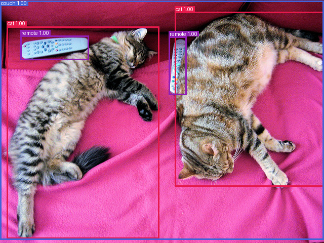
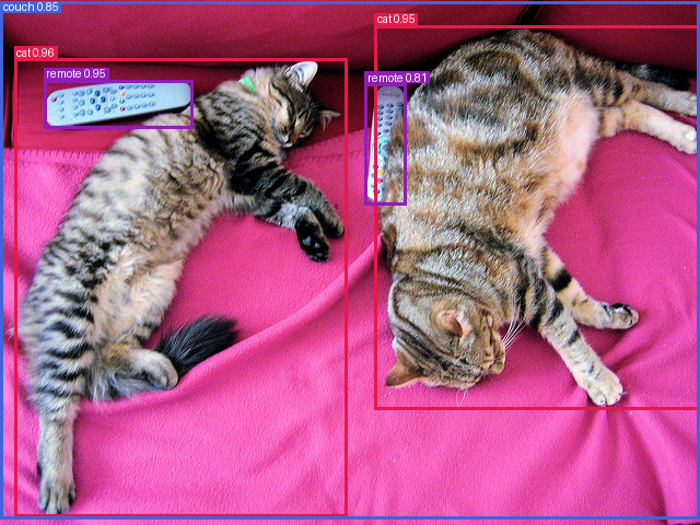
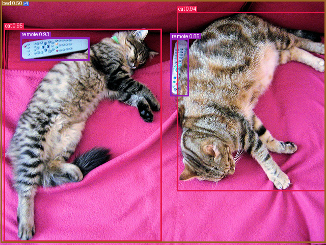
import urllib.request
from itertools import islice

from datasets import load_dataset
from IPython.display import display
from PIL import Image, ImageDraw

# The canonical COCO sample: two cats on a sofa with two remotes.
SAMPLE = DATA_DIR / "coco_cats.jpg"
if not SAMPLE.exists():
    urllib.request.urlretrieve("http://images.cocodataset.org/val2017/000000039769.jpg", SAMPLE)
image = Image.open(SAMPLE).convert("RGB")

# --- label normalisation -------------------------------------------------
# DETR/YOLOS carry the 91-entry COCO id list ("sofa", "tv"); RT-DETR/D-FINE/RF-DETR
# carry contiguous 80-class ids ("couch"). Compare by normalised NAME, never by id.
ALIASES = {"sofa": "couch", "tvmonitor": "tv", "aeroplane": "airplane",
           "motorbike": "motorcycle", "diningtable": "dining table",
           "pottedplant": "potted plant", "cellphone": "cell phone"}

def norm_label(name):
    "Lower-case a class name and fold the known cross-checkpoint synonyms."
    name = str(name).lower().strip()
    return ALIASES.get(name, name)

# --- the eval slice ------------------------------------------------------
N_EVAL = 24  # a smoke test, not a leaderboard (see section 12)
stream = load_dataset("detection-datasets/coco", split="val", streaming=True, cache_dir=HF_CACHE)
cat_feat = stream.features["objects"]["category"]
COCO80 = (cat_feat.feature if hasattr(cat_feat, "feature") else cat_feat).names

EVAL = []
for row in islice(stream, N_EVAL):  # streaming -> we pull a few MB, not the 800 MB val shard
    objs = row["objects"]
    EVAL.append({
        "image": row["image"].convert("RGB"),
        "boxes": np.asarray(objs["bbox"], dtype=np.float32).reshape(-1, 4),  # xyxy, absolute px
        "labels": [norm_label(COCO80[c]) for c in objs["category"]],
    })
del stream
free_memory()

print(f"{len(EVAL)} eval images, {sum(len(e['labels']) for e in EVAL)} ground-truth boxes")

# --- drawing (PIL, not matplotlib - ECharts is for charts, PIL for images) ---
PALETTE = ["#e6194b", "#3cb44b", "#4363d8", "#f58231", "#911eb4", "#42d4f4",
           "#f032e6", "#bfef45", "#fabed4", "#469990", "#dcbeff", "#9a6324"]

def draw_boxes(img, labels, boxes, scores=None, width=3):
    "Draw labelled boxes (xyxy) on a copy of a PIL image and return it."
    out = img.copy()
    d = ImageDraw.Draw(out)
    for i, (lab, box) in enumerate(zip(labels, boxes)):
        color = PALETTE[sum(map(ord, lab)) % len(PALETTE)]
        x0, y0, x1, y1 = (float(v) for v in box)
        d.rectangle([x0, y0, x1, y1], outline=color, width=width)
        text = lab if scores is None else f"{lab} {float(scores[i]):.2f}"
        tx, ty = x0 + 2, max(0.0, y0 - 12)
        bg = d.textbbox((tx, ty), text)
        d.rectangle([bg[0] - 2, bg[1] - 1, bg[2] + 2, bg[3] + 1], fill=color)
        d.text((tx, ty), text, fill="white")
    return out

# Ground truth of the first eval image - this is what the models are scored against.
display(draw_boxes(EVAL[0]["image"], EVAL[0]["labels"], EVAL[0]["boxes"]))


# --- inference helpers (used by every model section and by the benchmark) ---
@torch.inference_mode()
def predict(model, processor, images, threshold=0.5):
    """Run a transformers detector over PIL images -> [{labels, scores, boxes}, ...].

    Boxes come back xyxy in absolute pixels of the ORIGINAL image (that is what
    target_sizes buys you), and labels are normalised class-name strings, so
    outputs from any two checkpoints in this notebook are directly comparable.
    """
    out = []
    for img in images:
        inputs = processor(images=img, return_tensors="pt").to(device=device, dtype=dtype)
        res = model(**inputs)
        post = processor.post_process_object_detection(
            res, target_sizes=[(img.height, img.width)], threshold=threshold
        )[0]
        out.append({
            "labels": [norm_label(model.config.id2label[i]) for i in post["labels"].tolist()],
            "scores": post["scores"].float().cpu().numpy(),   # off the GPU before we free it
            "boxes": post["boxes"].float().cpu().numpy(),
        })
    return out

def show(pred, img, k=10):
    "Print the top-k detections and display the annotated image."
    order = np.argsort(-pred["scores"])[:k]
    for i in order:
        print(f"  {pred['labels'][i]:<14s} {pred['scores'][i]:.3f}  "
              f"{[round(float(v), 1) for v in pred['boxes'][i]]}")
    display(draw_boxes(img, [pred["labels"][i] for i in order],
                       [pred["boxes"][i] for i in order],
                       [pred["scores"][i] for i in order]))

24 eval images, 159 ground-truth boxes

8. DETR (the set-prediction original)

facebook/detr-resnet-50 (42M params, 42.0 AP) is the 2020 model that removed anchors and NMS: a ResNet-50 backbone, a 6+6-layer transformer encoder-decoder, 100 learned object queries, and a Hungarian-matched loss. It is not competitive on accuracy or speed any more, but it is the ancestor of every model in section 6’s top rows and the clearest thing to read.

Two DETR-specific quirks to know:

• Its classification head is a softmax over 91 classes + a “no-object” class, so scores are high-confidence and the sensible display threshold is 0.9. The focal-loss models below (RT-DETR, D-FINE, RF-DETR) use independent sigmoids, so their scores are lower and calibrated differently - 0.3-0.5 is the right display threshold there. Do not copy a threshold across model families.
• It is weak on small objects (one low-resolution feature map, global attention), which is exactly what Deformable DETR’s multi-scale sparse attention fixed.

---

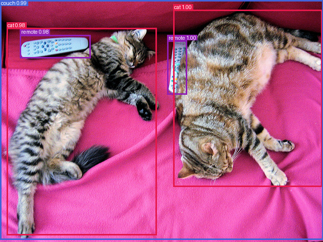
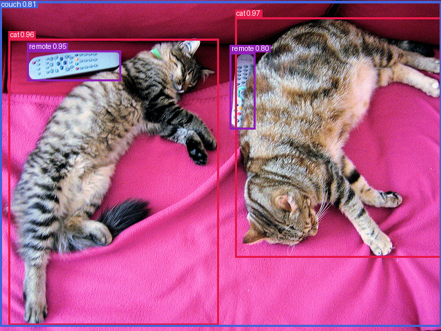
from transformers import AutoImageProcessor, AutoModelForObjectDetection

detr_id = "facebook/detr-resnet-50"
detr_proc = AutoImageProcessor.from_pretrained(detr_id, cache_dir=HF_CACHE)
detr = AutoModelForObjectDetection.from_pretrained(
    detr_id, cache_dir=HF_CACHE, dtype=dtype
).to(device).eval()
print(f"{sum(p.numel() for p in detr.parameters()) / 1e6:.1f}M params, "
      f"{detr.config.num_queries} object queries, {len(detr.config.id2label)} class ids")
vram("detr loaded")

predict(detr, detr_proc, [image], threshold=0.9)          # warm-up (CUDA autotune, kernel load)
t0 = time.perf_counter()
pred = predict(detr, detr_proc, [image], threshold=0.9)[0]  # softmax head -> high threshold
print(f"DETR-R50: {(time.perf_counter() - t0) * 1000:.0f} ms, {len(pred['labels'])} detections")
show(pred, image)

del detr, detr_proc, pred
free_memory()
vram("after detr")

[transformers] DetrForObjectDetection LOAD REPORT from: facebook/detr-resnet-50

Key                                                            | Status     |  | 

---------------------------------------------------------------+------------+--+-

model.backbone.model.layer1.0.downsample.1.num_batches_tracked | UNEXPECTED |  | 

model.backbone.model.layer4.0.downsample.1.num_batches_tracked | UNEXPECTED |  | 

model.backbone.model.layer3.0.downsample.1.num_batches_tracked | UNEXPECTED |  | 

model.backbone.model.layer2.0.downsample.1.num_batches_tracked | UNEXPECTED |  | 



Notes:

- UNEXPECTED:   can be ignored when loading from different task/architecture; not ok if you expect identical arch.

41.5M params, 100 object queries, 91 class ids
VRAM detr loaded           0.10 GB allocated /  0.11 GB reserved
DETR-R50: 29 ms, 5 detections
  cat            0.999  [13.2, 52.1, 314.1, 471.1]
  cat            0.999  [345.3, 23.9, 640.0, 368.7]
  remote         0.998  [40.2, 70.8, 175.6, 118.0]
  remote         0.996  [333.1, 72.5, 368.1, 187.6]
  couch          0.996  [0.0, 1.3, 639.7, 473.9]

VRAM after detr            0.01 GB allocated /  0.03 GB reserved

9. YOLOS (a plain ViT that detects)

hustvl/yolos-small (31M params, 36.1 AP) is the “You Only Look at One Sequence” model: a plain ViT with 100 detection tokens appended to the patch sequence, and nothing else - no CNN backbone, no FPN, no anchors, no NMS. It was a research statement (transfer a vanilla ViT to detection with minimal surgery) rather than a performance play, and its AP shows it.

It is here for two reasons: it is the clean demonstration that detection needs no convolutional inductive bias, and - despite the name - it is Apache 2.0 and transformers-native, unlike the Ultralytics YOLOs. Like DETR it uses a softmax head, so keep the threshold high.

---

yolos_id = "hustvl/yolos-small"
yolos_proc = AutoImageProcessor.from_pretrained(yolos_id, cache_dir=HF_CACHE)
yolos = AutoModelForObjectDetection.from_pretrained(
    yolos_id, cache_dir=HF_CACHE, dtype=dtype
).to(device).eval()
print(f"{sum(p.numel() for p in yolos.parameters()) / 1e6:.1f}M params (plain ViT, no CNN)")

predict(yolos, yolos_proc, [image], threshold=0.9)  # warm-up
t0 = time.perf_counter()
pred = predict(yolos, yolos_proc, [image], threshold=0.9)[0]
print(f"YOLOS-small: {(time.perf_counter() - t0) * 1000:.0f} ms, {len(pred['labels'])} detections")
show(pred, image)

del yolos, yolos_proc, pred
free_memory()
vram("after yolos")

30.7M params (plain ViT, no CNN)
YOLOS-small: 63 ms, 5 detections
  remote         0.999  [331.9, 80.6, 370.0, 188.0]
  cat            0.998  [343.4, 19.8, 638.4, 370.8]
  couch          0.987  [0.0, 0.0, 640.0, 475.8]
  cat            0.984  [13.1, 55.7, 310.9, 466.9]
  remote         0.979  [39.5, 69.4, 179.8, 116.0]

VRAM after yolos           0.01 GB allocated /  0.03 GB reserved

10. RT-DETRv2 (the production default)

PekingU/rtdetr_v2_r18vd (20M params, 48.1 AP) - Baidu’s real-time DETR, the model that first beat YOLO on the speed/accuracy front while staying NMS-free. A hybrid encoder decouples intra-scale attention from cross-scale fusion (cheap), and IoU-aware query selection seeds the decoder with good proposals (fast convergence). v2 adds selective multi-scale sampling and a discrete sampling operator that replaces grid_sample, which is the reason it exports cleanly to ONNX/TensorRT - the practical difference between a paper and a deployment.

Pick it when you want a boring, mature, well-exported detector. Larger siblings: rtdetr_v2_r34vd, rtdetr_v2_r50vd (53.4 AP), rtdetr_v2_r101vd. Note the processor resizes to 640x640 - feeding other sizes degrades accuracy.

---

rtdetr_id = "PekingU/rtdetr_v2_r18vd"
rtdetr_proc = AutoImageProcessor.from_pretrained(rtdetr_id, cache_dir=HF_CACHE)
rtdetr = AutoModelForObjectDetection.from_pretrained(
    rtdetr_id, cache_dir=HF_CACHE, dtype=dtype
).to(device).eval()
print(f"{sum(p.numel() for p in rtdetr.parameters()) / 1e6:.1f}M params, "
      f"{rtdetr.config.num_queries} queries, no NMS")

predict(rtdetr, rtdetr_proc, [image], threshold=0.5)  # warm-up
t0 = time.perf_counter()
pred = predict(rtdetr, rtdetr_proc, [image], threshold=0.5)[0]  # sigmoid head -> lower threshold
print(f"RT-DETRv2-R18: {(time.perf_counter() - t0) * 1000:.0f} ms, {len(pred['labels'])} detections")
show(pred, image)

del rtdetr, rtdetr_proc, pred
free_memory()
vram("after rt-detr")

20.2M params, 300 queries, no NMS
RT-DETRv2-R18: 23 ms, 6 detections
  cat            0.965  [341.2, 25.1, 640.0, 373.0]
  cat            0.960  [12.7, 56.4, 317.8, 471.5]
  remote         0.946  [40.0, 73.1, 175.6, 117.4]
  couch          0.862  [-0.2, 2.9, 640.0, 473.5]
  couch          0.814  [-0.2, 1.8, 640.0, 473.5]
  remote         0.796  [333.8, 76.4, 370.5, 187.5]

VRAM after rt-detr         0.01 GB allocated /  0.03 GB reserved

11. D-FINE (localisation specialist, tiny)

ustc-community/dfine-small-coco (10M params, 48.5 AP) beats the 20M RT-DETRv2-R18 with half the parameters. Its idea: stop regressing four scalar coordinates and instead predict a probability distribution over each box edge’s offset, refined iteratively across decoder layers (Fine-grained Distribution Refinement), with the sharper deep-layer distributions distilled back into the shallow layers (GO-LSD). Because it optimises where the edge probably is rather than a point estimate, it wins disproportionately at high IoU thresholds - which is exactly what AP@[.50:.95] rewards.

The family runs dfine-nano-coco (3.8M) to dfine-xlarge-coco (63M, 55.8 AP). Checkpoints suffixed -obj365 are Objects365-pretrained and -obj2coco are Objects365-pretrained then COCO-finetuned (D-FINE-L/X reach 57.1 / 59.3 AP that way) - a free 3 AP if you can spare the download.

---

dfine_id = "ustc-community/dfine-small-coco"
dfine_proc = AutoImageProcessor.from_pretrained(dfine_id, cache_dir=HF_CACHE)
dfine = AutoModelForObjectDetection.from_pretrained(
    dfine_id, cache_dir=HF_CACHE, dtype=dtype
).to(device).eval()
print(f"{sum(p.numel() for p in dfine.parameters()) / 1e6:.1f}M params, "
      f"max_num_bins={dfine.config.max_num_bins} (the corner-offset distribution)")

predict(dfine, dfine_proc, [image], threshold=0.5)  # warm-up
t0 = time.perf_counter()
pred = predict(dfine, dfine_proc, [image], threshold=0.5)[0]
print(f"D-FINE-S: {(time.perf_counter() - t0) * 1000:.0f} ms, {len(pred['labels'])} detections")
show(pred, image)

del dfine, dfine_proc, pred
free_memory()
vram("after d-fine")

10.3M params, max_num_bins=32 (the corner-offset distribution)
D-FINE-S: 13 ms, 5 detections
  cat            0.962  [13.3, 53.9, 317.0, 472.0]
  remote         0.954  [40.3, 73.0, 176.1, 117.8]
  cat            0.953  [342.5, 23.4, 640.0, 374.5]
  couch          0.854  [0.6, 1.2, 639.5, 474.8]
  remote         0.813  [333.5, 76.7, 371.0, 187.8]

VRAM after d-fine          0.01 GB allocated /  0.03 GB reserved

12. RF-DETR (the mid-2026 state of the art)

Roboflow/rf-detr-medium (34M params) - the ICLR 2026 model that currently leads the real-time Pareto front. A DINOv2-with-registers ViT backbone (windowed/full attention alternation), a C2f-style multi-scale projector, and a shallow deformable DETR decoder, with the whole configuration chosen by weight-sharing neural architecture search over the accuracy/latency frontier instead of by hand. Group-DETR training (parallel decoder copies) gives it fast convergence.

The NAS result is worth reading off the configs: nano / medium / large differ by input resolution (384 / 576 / 704) and decoder depth (2 / 4 / 4), not by channel width - which is why the whole family sits at ~30-34M params. Scaling a detector by resolution rather than by width is the opposite of the usual n/s/m/l/x recipe, and it is where the latency wins come from.

Why it matters beyond one more AP point: the DINOv2 backbone is a self-supervised foundation model, so RF-DETR transfers far better than a COCO-supervised CNN - it is the first real-time detector past 60 mAP on RF100-VL, the benchmark that simulates your actual dataset (X-ray, aerial, industrial) rather than tourist photos. That is what makes it the default when you plan to fine-tune. Family: rf-detr-nano (48.0 AP) through rf-detr-large, plus Roboflow/rf-detr-seg-medium for instance masks (see 03_Image_Segmentation). Apache 2.0.

---

rfdetr_id = "Roboflow/rf-detr-medium"
rfdetr_proc = AutoImageProcessor.from_pretrained(rfdetr_id, cache_dir=HF_CACHE)
rfdetr = AutoModelForObjectDetection.from_pretrained(
    rfdetr_id, cache_dir=HF_CACHE, dtype=dtype
).to(device).eval()
print(f"{sum(p.numel() for p in rfdetr.parameters()) / 1e6:.1f}M params, "
      f"{rfdetr.config.decoder_layers}-layer decoder, "
      f"{rfdetr.config.backbone_config.image_size}px DINOv2 backbone")

predict(rfdetr, rfdetr_proc, [image], threshold=0.5)  # warm-up
t0 = time.perf_counter()
pred = predict(rfdetr, rfdetr_proc, [image], threshold=0.5)[0]
print(f"RF-DETR-medium: {(time.perf_counter() - t0) * 1000:.0f} ms, {len(pred['labels'])} detections")
show(pred, image)

del rfdetr, rfdetr_proc, pred
free_memory()
vram("after rf-detr")

33.7M params, 4-layer decoder, 576px DINOv2 backbone
RF-DETR-medium: 15 ms, 6 detections
  cat            0.947  [7.6, 56.0, 317.0, 473.8]
  cat            0.940  [347.5, 23.3, 639.5, 374.5]
  remote         0.931  [40.1, 73.1, 175.1, 118.2]
  remote         0.854  [334.5, 76.8, 370.5, 188.1]
  couch          0.536  [1.6, 0.5, 639.0, 475.2]
  bed            0.504  [1.6, 0.5, 639.0, 475.2]

VRAM after rf-detr         0.01 GB allocated /  0.03 GB reserved

13. Head-to-head Benchmark

All five detectors on the same 24 COCO val2017 images, the same ground truth, and the same metric - real COCO mAP@[.50:.95] (101-point interpolation, per class then averaged) computed with the iou_matrix / ap_101 functions from section 4, plus AP50 and end-to-end latency per image. Models are loaded, measured and freed one at a time, so VRAM returns to baseline between rows.

Two protocol details that matter:

• We predict with a threshold of 0.05, not the 0.5 used for display. AP integrates over the whole ranked list; thresholding first would truncate the recall axis and understate every model.
• Latency is wall-clock per image, batch size 1, fp16 on GPU, measured after a warm-up pass, and it includes preprocessing and post-processing. It is not the number the papers quote (those are TensorRT, often on a T4/A100), so read the ordering, not the absolute values.

This is a smoke test, not a leaderboard. 24 images out of 5000 gives a mAP with several points of noise, and rare classes appear zero or once. Published COCO numbers (DETR 42.0, YOLOS-S 36.1, RT-DETRv2-R18 48.1, D-FINE-S 48.5) are the ground truth; the point here is to see the shape of the ranking reproduce on your own hardware, and to see how much latency you pay for it.

---

def coco_map(preds, gts, iou_thrs=np.arange(0.5, 1.0, 0.05)):
    """COCO mAP over a list of per-image predictions and ground truths.

    Averages 101-point AP over the given IoU thresholds, per class, then over the
    classes that actually appear in the ground truth. Matching is greedy in
    confidence order with one-to-one assignment (a second box on a matched object
    is a duplicate = false positive), exactly as pycocotools does it.
    """
    classes = sorted({lab for g in gts for lab in g["labels"]})
    aps = []
    for cls in classes:
        gt_boxes, n_gt = [], 0
        for g in gts:
            keep = [j for j, lab in enumerate(g["labels"]) if lab == cls]
            gt_boxes.append(g["boxes"][keep] if keep else np.zeros((0, 4), dtype=np.float32))
            n_gt += len(keep)
        dets = [(float(p["scores"][j]), i, p["boxes"][j])
                for i, p in enumerate(preds)
                for j, lab in enumerate(p["labels"]) if lab == cls]
        if n_gt == 0:
            continue
        dets.sort(key=lambda d: -d[0])
        per_thr = []
        for thr in iou_thrs:
            used = [np.zeros(len(g), dtype=bool) for g in gt_boxes]
            tp, fp = np.zeros(len(dets)), np.zeros(len(dets))
            for k, (_, img_i, box) in enumerate(dets):
                g = gt_boxes[img_i]
                if len(g) == 0:
                    fp[k] = 1
                    continue
                ious = iou_matrix(box[None, :], g)[0]
                best = int(ious.argmax())
                if ious[best] >= thr and not used[img_i][best]:
                    tp[k], used[img_i][best] = 1, True
                else:
                    fp[k] = 1
            per_thr.append(ap_101(tp, fp, n_gt))
        aps.append(float(np.mean(per_thr)))
    return float(np.mean(aps)) if aps else 0.0


# Sanity check: the ground truth scored against itself must be a perfect 1.0.
perfect = [{"labels": e["labels"], "boxes": e["boxes"],
            "scores": np.ones(len(e["labels"]))} for e in EVAL]
print("mAP of the ground truth against itself:", round(coco_map(perfect, EVAL), 4))
del perfect

mAP of the ground truth against itself: 1.0

import pandas as pd

MODELS = {
    "DETR-R50": "facebook/detr-resnet-50",
    "YOLOS-small": "hustvl/yolos-small",
    "RT-DETRv2-R18": "PekingU/rtdetr_v2_r18vd",
    "D-FINE-S": "ustc-community/dfine-small-coco",
    "RF-DETR-medium": "Roboflow/rf-detr-medium",
}

results = {}
images = [e["image"] for e in EVAL]

for name, model_id in MODELS.items():
    proc = AutoImageProcessor.from_pretrained(model_id, cache_dir=HF_CACHE)
    model = AutoModelForObjectDetection.from_pretrained(
        model_id, cache_dir=HF_CACHE, dtype=dtype
    ).to(device).eval()
    n_params = sum(p.numel() for p in model.parameters()) / 1e6

    predict(model, proc, images[:1], threshold=0.5)  # warm-up, not timed
    t0 = time.perf_counter()
    preds = predict(model, proc, images, threshold=0.05)  # low threshold: AP wants the full list
    ms = (time.perf_counter() - t0) / len(images) * 1000

    results[name] = {
        "params_M": round(n_params, 1),
        "mAP@[.50:.95]": round(coco_map(preds, EVAL), 4),
        "AP50": round(coco_map(preds, EVAL, iou_thrs=np.array([0.5])), 4),
        "ms_per_image": round(ms, 1),
        "boxes@0.5": int(sum((p["scores"] >= 0.5).sum() for p in preds)),
    }
    print(f"{name:16s} {results[name]}")

    del model, proc, preds  # free before loading the next - never two detectors live at once
    free_memory()

vram("after benchmark")

df = (pd.DataFrame(results).T
      .sort_values("mAP@[.50:.95]", ascending=False)
      .rename_axis("model").reset_index())
df

[transformers] DetrForObjectDetection LOAD REPORT from: facebook/detr-resnet-50

Key                                                            | Status     |  | 

---------------------------------------------------------------+------------+--+-

model.backbone.model.layer1.0.downsample.1.num_batches_tracked | UNEXPECTED |  | 

model.backbone.model.layer4.0.downsample.1.num_batches_tracked | UNEXPECTED |  | 

model.backbone.model.layer3.0.downsample.1.num_batches_tracked | UNEXPECTED |  | 

model.backbone.model.layer2.0.downsample.1.num_batches_tracked | UNEXPECTED |  | 



Notes:

- UNEXPECTED:   can be ignored when loading from different task/architecture; not ok if you expect identical arch.

DETR-R50         {'params_M': 41.5, 'mAP@[.50:.95]': 0.5222, 'AP50': 0.7098, 'ms_per_image': 31.0, 'boxes@0.5': 279}

YOLOS-small      {'params_M': 30.7, 'mAP@[.50:.95]': 0.468, 'AP50': 0.5903, 'ms_per_image': 33.2, 'boxes@0.5': 309}

RT-DETRv2-R18    {'params_M': 20.2, 'mAP@[.50:.95]': 0.6231, 'AP50': 0.757, 'ms_per_image': 13.6, 'boxes@0.5': 147}

D-FINE-S         {'params_M': 10.3, 'mAP@[.50:.95]': 0.6499, 'AP50': 0.7916, 'ms_per_image': 24.4, 'boxes@0.5': 145}

RF-DETR-medium   {'params_M': 33.7, 'mAP@[.50:.95]': 0.6639, 'AP50': 0.8165, 'ms_per_image': 23.2, 'boxes@0.5': 112}
VRAM after benchmark       0.01 GB allocated /  0.03 GB reserved

	model	params_M	mAP@[.50:.95]	AP50	ms_per_image	boxes@0.5
0	RF-DETR-medium	33.7	0.6639	0.8165	23.2	112.0
1	D-FINE-S	10.3	0.6499	0.7916	24.4	145.0
2	RT-DETRv2-R18	20.2	0.6231	0.7570	13.6	147.0
3	DETR-R50	41.5	0.5222	0.7098	31.0	279.0
4	YOLOS-small	30.7	0.4680	0.5903	33.2	309.0

from pyecharts import options as opts
from pyecharts.charts import Bar, Scatter

names = list(df["model"])

bar = (
    Bar()
    .add_xaxis(names)
    .add_yaxis("mAP@[.50:.95]", [round(float(v), 3) for v in df["mAP@[.50:.95]"]])
    .add_yaxis("AP50", [round(float(v), 3) for v in df["AP50"]])
    .set_global_opts(
        title_opts=opts.TitleOpts(
            title="COCO mAP on 24 val2017 images",
            subtitle="Smoke test on an RTX 3060 (fp16, batch 1) - not a leaderboard",
        ),
        xaxis_opts=opts.AxisOpts(name="model", axislabel_opts=opts.LabelOpts(rotate=20)),
        yaxis_opts=opts.AxisOpts(name="AP"),
        tooltip_opts=opts.TooltipOpts(trigger="axis"),
    )
)
bar.render_notebook()

# The chart that actually decides a deployment: accuracy against latency.
scatter = Scatter().add_xaxis([round(float(v), 1) for v in df["ms_per_image"]])
for name, ms, ap in zip(df["model"], df["ms_per_image"], df["mAP@[.50:.95]"]):
    scatter.add_yaxis(
        name,
        [[round(float(ms), 1), round(float(ap), 3)]],
        symbol_size=18,
        label_opts=opts.LabelOpts(is_show=False),
    )
scatter.set_global_opts(
    title_opts=opts.TitleOpts(
        title="Speed / accuracy trade-off",
        subtitle="end-to-end ms per image (preprocess + forward + post-process), up-left is better",
    ),
    xaxis_opts=opts.AxisOpts(type_="value", name="ms per image"),
    yaxis_opts=opts.AxisOpts(type_="value", name="mAP@[.50:.95]"),
    tooltip_opts=opts.TooltipOpts(trigger="item"),
)
scatter.render_notebook()

14. Real-time Webcam Demo

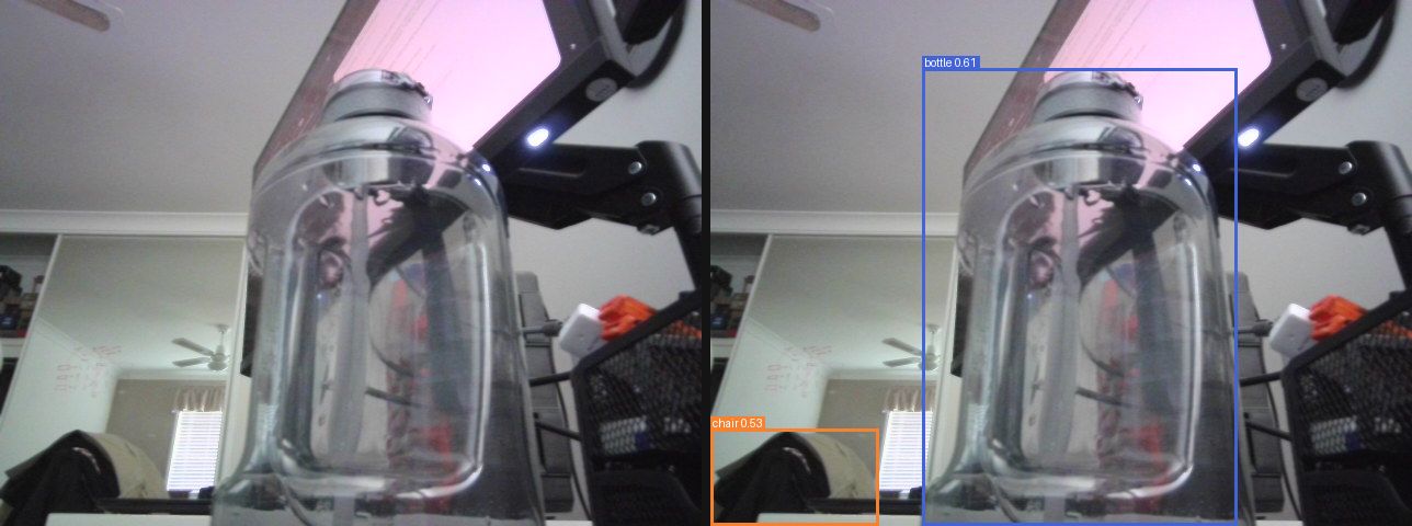
Detection is the one CV task that is genuinely fun live. This grabs frames from a webcam with OpenCV and runs rf-detr-nano (30M params) on each one. On a headless server there is no camera, so the cell reports that and skips cleanly.

For real video work you would add a tracker on top (ByteTrack / BoT-SORT associate boxes across frames into identities), export the model to TensorRT or ONNX Runtime, and batch frames - a Python loop like the one below is not what “real-time” means in production.

---

# opencv-python-headless is a project dependency; the headless build captures from
# V4L2 fine, it only drops the GUI windows.
import io
import time

import cv2
import numpy as np
import torch
from IPython.display import Image as IPyImage
from IPython.display import Pretty, display
from PIL import Image, ImageDraw, ImageFont

CAM = 0              # /dev/video0
WARMUP = 10          # throwaway reads - auto-exposure and white balance need to settle
STREAM_SECONDS = 15  # how long a live demo runs; interrupt the kernel to stop early


def bootstrap(*names, notebook, sections):
    """Make this demo runnable on a cold kernel, without duplicating the notebook.

    The demo builds on the notebook's setup and helper cells. Instead of making you
    run them by hand - or copying them in here and letting the copies drift - this
    reads the notebook file and executes those sections itself, and only when a name
    is actually missing. Run the notebook top to bottom and it does nothing at all.
    It stops as soon as every required name exists, so trailing benchmark cells in a
    section are not run.
    """
    if all(n in globals() for n in names):
        return
    import json
    from pathlib import Path

    from IPython.utils.capture import capture_output

    path = Path(notebook)
    if not path.exists():
        raise NameError(
            f"this demo needs {', '.join(n for n in names if n not in globals())}, and cannot "
            f"find {notebook} to bootstrap from (cwd is {Path.cwd()}, expected the notebook's "
            f"own directory). Run section(s) {'; '.join(sections)} by hand instead."
        )
    print(f"cold start: running {'; '.join(sections)} from {notebook} (output suppressed)")
    heading = None
    for cell in json.loads(path.read_text())["cells"]:
        src = "".join(cell["source"])
        if cell["cell_type"] == "markdown" and src.lstrip().startswith("## "):
            heading = src.lstrip().splitlines()[0][3:].strip()
            continue
        if cell["cell_type"] != "code" or not heading or "def bootstrap(" in src:
            continue
        if not any(heading.startswith(s) for s in sections):
            continue
        code = "".join("" if l.lstrip().startswith(("%", "!")) else l
                       for l in src.splitlines(keepends=True))
        # The setup cells print tables and display sample images. This demo only
        # wants the live stream, so swallow their output - errors still propagate.
        with capture_output():
            exec(compile(code, f"{notebook} [{heading}]", "exec"), globals())
        if all(n in globals() for n in names):
            break
    still = [n for n in names if n not in globals()]
    if still:
        raise NameError(f"bootstrapped {'; '.join(sections)} but {', '.join(still)} "
                        "are still undefined - the notebook layout may have changed.")


def open_camera(index=CAM, width=640, height=480, auto_exposure=True, exposure=150):
    "Open a V4L2 webcam in MJPEG mode, let it settle, and return the capture handle."
    cap = cv2.VideoCapture(index, cv2.CAP_V4L2)
    if not cap.isOpened():
        raise RuntimeError(
            f"/dev/video{index} did not open - no camera attached, "
            "or it is not passed through into this container"
        )
    cap.set(cv2.CAP_PROP_FOURCC, cv2.VideoWriter.fourcc(*"MJPG"))  # MJPEG unlocks the higher modes
    cap.set(cv2.CAP_PROP_FRAME_WIDTH, width)
    cap.set(cv2.CAP_PROP_FRAME_HEIGHT, height)
    # UVC exposure is DEVICE state and persists between processes: if anything left
    # this camera in manual mode, every frame comes back dark and never adapts
    # (measured here: mean 13/255 stuck, vs 109/255 on auto). So ask for the mode
    # explicitly instead of inheriting whatever the last program set.
    #   auto (3): correct brightness, but a dim room throttles the sensor to 15 FPS
    #   manual (1): locked 30 FPS, at whatever `exposure` level suits your lighting
    cap.set(cv2.CAP_PROP_AUTO_EXPOSURE, 3 if auto_exposure else 1)
    if not auto_exposure:
        cap.set(cv2.CAP_PROP_EXPOSURE, exposure)
    # Deliberately no CAP_PROP_BUFFERSIZE: on the V4L2 backend it HALVES the
    # delivered frame rate (measured here: 67 -> 134 ms per read) and does not make
    # frames any fresher.
    for _ in range(WARMUP):
        if not cap.read()[0]:
            cap.release()
            raise RuntimeError(f"/dev/video{index} opened but delivered no frames")
    return cap


def grab(cap):
    "Read one frame off an open camera as an RGB PIL image (OpenCV hands back BGR)."
    ok, frame = cap.read()
    if not ok:
        raise RuntimeError("failed to read a frame")
    return Image.fromarray(cv2.cvtColor(frame, cv2.COLOR_BGR2RGB))


def capture_frame(**kw):
    "Open the camera, grab one settled frame, and release the device."
    cap = open_camera(**kw)
    try:
        return grab(cap)
    finally:
        cap.release()


_FONT = ImageFont.load_default(size=15)


def draw_lines(img, lines, pad=6):
    "Burn a few lines of text into a band across the top of a copy of `img`."
    out = img.convert("RGB").copy()
    d = ImageDraw.Draw(out)
    d.rectangle([0, 0, out.width, 18 * len(lines) + 2 * pad], fill=(0, 0, 0))
    for i, line in enumerate(lines):
        d.text((pad, pad + 18 * i), line, fill=(255, 255, 255), font=_FONT)
    return out


def pair_view(left, right, gap=8):
    "Raw frame and annotated frame side by side on one canvas - the live view."
    right = right.convert("RGB")
    if right.size != left.size:
        right = right.resize(left.size)
    canvas = Image.new("RGB", (left.width * 2 + gap, left.height), (20, 20, 20))
    canvas.paste(left.convert("RGB"), (0, 0))
    canvas.paste(right, (left.width + gap, 0))
    return canvas


def _jpeg(img, quality=80):
    "Encode a PIL image to JPEG bytes - what actually goes over the wire each frame."
    buf = io.BytesIO()
    img.convert("RGB").save(buf, format="JPEG", quality=quality)
    return buf.getvalue()


def live_stream(annotate, seconds=STREAM_SECONDS, width=640, height=480):
    """Stream `raw | annotated` into the notebook output until `seconds` elapse.

    `annotate(rgb)` returns `(annotated_image, info_string)`. The image and the
    status line each own a display handle and update in place, so this needs no GUI
    and no `cv2.imshow` - it works over JupyterLab against a headless container.
    Interrupt the kernel (the stop button) to end early; the camera is still released.
    """
    cap = open_camera(width=width, height=height)
    view = status = None  # created from the FIRST real frame, so no placeholder flashes up
    n, t0 = 0, time.perf_counter()
    try:
        while time.perf_counter() - t0 < seconds:
            rgb = grab(cap)
            annotated, info = annotate(rgb)
            n += 1
            frame = IPyImage(data=_jpeg(pair_view(rgb, annotated)))
            line = Pretty(f"frame {n:4d}   {n / (time.perf_counter() - t0):5.1f} FPS   {info}")
            if view is None:
                view = display(frame, display_id=True)
                status = display(line, display_id=True)
            else:
                view.update(frame)
                status.update(line)
    except KeyboardInterrupt:
        if status is not None:
            status.update(Pretty(f"stopped at frame {n}"))
    finally:
        cap.release()  # always hand the device back
    elapsed = time.perf_counter() - t0
    print(f"{n} frames in {elapsed:.1f}s -> {n / max(elapsed, 1e-9):.1f} FPS end-to-end "
          "(camera + model + JPEG encode)")


def preview(seconds=5, width=640, height=480):
    "Stream the raw camera so you can frame the shot, then return the final frame."
    cap = open_camera(width=width, height=height)
    view = status = None  # created from the FIRST real frame, so no placeholder flashes up
    last, n, t0 = None, 0, time.perf_counter()
    try:
        while time.perf_counter() - t0 < seconds:
            last = grab(cap)
            n += 1
            frame = IPyImage(data=_jpeg(last))
            line = Pretty(f"framing - {seconds - (time.perf_counter() - t0):4.1f}s left, "
                          f"{n} frames (the last one is the one that gets used)")
            if view is None:
                view = display(frame, display_id=True)
                status = display(line, display_id=True)
            else:
                view.update(frame)
                status.update(line)
    except KeyboardInterrupt:
        pass
    finally:
        cap.release()
    if status is not None:
        status.update(Pretty(f"captured the last of {n} frames"))
    return last


from transformers import AutoImageProcessor, AutoModelForObjectDetection

# Everything below builds on the notebook's setup and helper cells.
bootstrap("device", "dtype", "HF_CACHE", "predict", "draw_boxes", "free_memory", "vram",
          notebook="02_Object_Detection.ipynb",
          sections=["4. Evaluation Metrics", "7. Setup"])



THRESH = 0.5

demo_id = "Roboflow/rf-detr-nano"  # smallest of the SOTA family - fastest per frame
demo_proc = AutoImageProcessor.from_pretrained(demo_id, cache_dir=HF_CACHE)
demo = AutoModelForObjectDetection.from_pretrained(
    demo_id, cache_dir=HF_CACHE, dtype=dtype
).to(device).eval()


def annotate(rgb):
    "One frame -> (frame with boxes drawn, how many things the model found)."
    pred = predict(demo, demo_proc, [rgb], threshold=THRESH)[0]
    boxed = draw_boxes(rgb, pred["labels"], pred["boxes"], pred["scores"])
    names = ", ".join(sorted(set(pred["labels"]))[:4]) or "nothing over threshold"
    return boxed, f"{len(pred['labels']):2d} detections   {names}"


live_stream(annotate)

del demo, demo_proc
free_memory()
vram("final")

frame  224    14.9 FPS    2 detections   bottle, chair

224 frames in 15.0s -> 14.9 FPS end-to-end (camera + model + JPEG encode)
VRAM final                 0.01 GB allocated /  0.02 GB reserved

15. Common Frameworks

Object detection has the most fragmented ecosystem in this folder, and the fragmentation is mostly licensing. The fastest and best-known models - the YOLO line - ship under AGPL-3.0 through a single vendor package, while the transformers-native DETR descendants are Apache 2.0. That choice is made at the start of a project and is expensive to reverse, so it belongs in the table rather than in a footnote.

Framework	Layer	What it gives you	License	Reach for it when
transformers	modelling	DETR, RT-DETRv2, D-FINE, RF-DETR and YOLOS behind AutoModelForObjectDetection, with COCO-format annotations accepted directly by the processor	Apache 2.0	Default, and in 2026 genuinely competitive. The license story alone is worth the switch
Ultralytics (YOLO11 / YOLO26)	modelling	The best-documented training and export experience in detection, and a large community	AGPL-3.0 (copyleft - it reaches your service unless you buy a commercial license)	You are prototyping, doing research, or you have bought the license. Read it before it is load-bearing
MMDetection / Detectron2	modelling	The widest zoo of the CNN era - Faster R-CNN, RTMDet, Cascade R-CNN - with reference training code	Apache 2.0	You need one exact architecture from a paper, or you are reproducing a published baseline
Roboflow supervision	data	Box/mask utilities that the model libraries all leave out: NMS, annotation drawing, zone counting, tracker glue	MIT	Always. Every detection project rewrites these badly at least once
FiftyOne + CVAT / Label Studio	data	Annotation, and - more importantly - per-image error analysis: which boxes were missed, which were duplicated, which classes swap	Apache 2.0 / MIT	Always. mAP tells you a model got worse; these tell you why
SAHI	data	Sliced inference: tile a large image, detect per tile, merge - the standard fix for small objects	MIT	Objects under ~32 px, aerial or document imagery. Cheaper and more effective than a bigger model
ONNX Runtime / TensorRT / OpenVINO	inference runtime	3-10x on the same weights; onnx-community/rfdetr_*-ONNX and dfine_*-ONNX are pre-exported	MIT / Apache 2.0 (TensorRT SDK proprietary)	Deployment, always. RT-DETRv2’s discrete sampling operator exists specifically to make this export painless
Triton Inference Server / DeepStream	serving	Batched serving, and in DeepStream’s case a full decode-to-detect-to-track video pipeline on GPU	BSD-3 / proprietary	Many camera streams at once. Decoding video is often the real bottleneck, not the model
pycocotools + torchmetrics	evaluation	The reference mAP implementation, per-IoU and per-size breakdowns	BSD-2 / Apache 2.0	Always, and read AP_small separately - the aggregate hides exactly the failure you are most likely to have

The 2026 default stack is transformers with RF-DETR or D-FINE, supervision for everything around the model, SAHI if the objects are small, and ONNX Runtime or TensorRT to deploy. The Apache-2.0 path is now fast enough that AGPL is a choice rather than a necessity.

The common wrong turn is picking a model on COCO mAP. COCO predicts almost nothing about your domain; transfer from a few hundred of your own boxes does, and an Objects365-pretrained checkpoint transfers noticeably better than a COCO-only one. The second is discovering the Ultralytics license after the model is embedded in a product.

---

16. Going Further

• Fine-tuning is the whole game. COCO mAP predicts almost nothing about your domain; what matters is how well a checkpoint transfers from a few hundred of your own boxes. Start from the official transformers object-detection examples (Trainer or Accelerate) and the object detection task guide; pass your COCO-format annotations straight to the image processor (format="coco_detection"), and supply labels as a list of dicts with class_labels + boxes (cxcywh, normalised). Prefer an Objects365-pretrained checkpoint (ustc-community/dfine-*-obj2coco) or RF-DETR as the starting point - both transfer noticeably better than a COCO-only CNN.
• Small objects. If your objects are under ~32 px, the fix is rarely a bigger model: tile the image (SAHI-style sliced inference), raise the input resolution, and check that your backbone still has a stride-8 feature map. Read AP_small, not AP.
• Related notebooks. 13_Zero_Shot_Object_Detection (OWLv2 / Grounding DINO - boxes from text prompts, no retraining), 03_Image_Segmentation (add pixel masks; Roboflow/rf-detr-seg-medium is the same model with a mask head), 12_Mask_Generation (SAM - promptable, class-agnostic masks, often chained after a detector), 17_Keypoint_Detection (pose inside each box), 01_Image_Classification (the single-label ancestor).

References

• DETR: End-to-End Object Detection with Transformers (Carion et al., 2020)
• Deformable DETR (Zhu et al., 2021) and Focal Loss / RetinaNet (Lin et al., 2017)
• RT-DETR: DETRs Beat YOLOs on Real-time Object Detection (Zhao et al., 2023) and RT-DETRv2 (2024)
• D-FINE: Redefine Regression as Fine-grained Distribution Refinement (2024)
• DEIMv2: Real-Time Object Detection Meets DINOv3 (2025)
• RF-DETR: Neural Architecture Search for Real-Time Detection Transformers (ICLR 2026)
• Roboflow100-VL: a multi-domain detection benchmark (NeurIPS 2025) and Papers with Code: real-time detection on COCO
• COCO detection evaluation protocol and Ultralytics AGPL-3.0 license

---