# import libraries
import numpy as np
import matplotlib.pyplot as plt
import pandas as pd
import seaborn as snsL1 and L2 Regularization
L1 and L2 Regularization
# Suppress Warnings for clean notebook
import warnings
warnings.filterwarnings('ignore')
We are going to use Melbourne House Price Dataset where we’ll predict House Predictions based on various features. #### The Dataset Link is https://www.kaggle.com/anthonypino/melbourne-housing-market
# read dataset
dataset_og = pd.read_csv('./Data/Melbourne_housing_FULL.csv')dataset_og.head()| Suburb | Address | Rooms | Type | Price | Method | SellerG | Date | Distance | Postcode | ... | Bathroom | Car | Landsize | BuildingArea | YearBuilt | CouncilArea | Lattitude | Longtitude | Regionname | Propertycount | |
|---|---|---|---|---|---|---|---|---|---|---|---|---|---|---|---|---|---|---|---|---|---|
| 0 | Abbotsford | 68 Studley St | 2 | h | NaN | SS | Jellis | 3/09/2016 | 2.5 | 3067.0 | ... | 1.0 | 1.0 | 126.0 | NaN | NaN | Yarra City Council | -37.8014 | 144.9958 | Northern Metropolitan | 4019.0 |
| 1 | Abbotsford | 85 Turner St | 2 | h | 1480000.0 | S | Biggin | 3/12/2016 | 2.5 | 3067.0 | ... | 1.0 | 1.0 | 202.0 | NaN | NaN | Yarra City Council | -37.7996 | 144.9984 | Northern Metropolitan | 4019.0 |
| 2 | Abbotsford | 25 Bloomburg St | 2 | h | 1035000.0 | S | Biggin | 4/02/2016 | 2.5 | 3067.0 | ... | 1.0 | 0.0 | 156.0 | 79.0 | 1900.0 | Yarra City Council | -37.8079 | 144.9934 | Northern Metropolitan | 4019.0 |
| 3 | Abbotsford | 18/659 Victoria St | 3 | u | NaN | VB | Rounds | 4/02/2016 | 2.5 | 3067.0 | ... | 2.0 | 1.0 | 0.0 | NaN | NaN | Yarra City Council | -37.8114 | 145.0116 | Northern Metropolitan | 4019.0 |
| 4 | Abbotsford | 5 Charles St | 3 | h | 1465000.0 | SP | Biggin | 4/03/2017 | 2.5 | 3067.0 | ... | 2.0 | 0.0 | 134.0 | 150.0 | 1900.0 | Yarra City Council | -37.8093 | 144.9944 | Northern Metropolitan | 4019.0 |
5 rows × 21 columns
dataset_og.nunique()Suburb 351
Address 34009
Rooms 12
Type 3
Price 2871
Method 9
SellerG 388
Date 78
Distance 215
Postcode 211
Bedroom2 15
Bathroom 11
Car 15
Landsize 1684
BuildingArea 740
YearBuilt 160
CouncilArea 33
Lattitude 13402
Longtitude 14524
Regionname 8
Propertycount 342
dtype: int64# let's use limited columns which makes more sense for serving our purpose
cols_to_use = ['Suburb', 'Rooms', 'Type', 'Method', 'SellerG', 'Regionname', 'Propertycount',
'Distance', 'CouncilArea', 'Bedroom2', 'Bathroom', 'Car', 'Landsize', 'BuildingArea', 'Price']
dataset = dataset_og[cols_to_use]dataset.head()| Suburb | Rooms | Type | Method | SellerG | Regionname | Propertycount | Distance | CouncilArea | Bedroom2 | Bathroom | Car | Landsize | BuildingArea | Price | |
|---|---|---|---|---|---|---|---|---|---|---|---|---|---|---|---|
| 0 | Abbotsford | 2 | h | SS | Jellis | Northern Metropolitan | 4019.0 | 2.5 | Yarra City Council | 2.0 | 1.0 | 1.0 | 126.0 | NaN | NaN |
| 1 | Abbotsford | 2 | h | S | Biggin | Northern Metropolitan | 4019.0 | 2.5 | Yarra City Council | 2.0 | 1.0 | 1.0 | 202.0 | NaN | 1480000.0 |
| 2 | Abbotsford | 2 | h | S | Biggin | Northern Metropolitan | 4019.0 | 2.5 | Yarra City Council | 2.0 | 1.0 | 0.0 | 156.0 | 79.0 | 1035000.0 |
| 3 | Abbotsford | 3 | u | VB | Rounds | Northern Metropolitan | 4019.0 | 2.5 | Yarra City Council | 3.0 | 2.0 | 1.0 | 0.0 | NaN | NaN |
| 4 | Abbotsford | 3 | h | SP | Biggin | Northern Metropolitan | 4019.0 | 2.5 | Yarra City Council | 3.0 | 2.0 | 0.0 | 134.0 | 150.0 | 1465000.0 |
dataset.shape(34857, 15)Checking for Nan values
dataset.isna().sum()Suburb 0
Rooms 0
Type 0
Method 0
SellerG 0
Regionname 3
Propertycount 3
Distance 1
CouncilArea 3
Bedroom2 8217
Bathroom 8226
Car 8728
Landsize 11810
BuildingArea 21115
Price 7610
dtype: int64#from sklearn.preprocessing import LabelEncoder
# Fit and transform the dates to numerical labels
#dataset['Date'] = LabelEncoder().fit_transform(dataset['Date'])Handling Missing values
# Some feature's missing values can be treated as zero (another class for NA values or absence of that feature)
# like 0 for Propertycount, Bedroom2 will refer to other class of NA values
# like 0 for Car feature will mean that there's no car parking feature with house
cols_to_fill_zero = ['Propertycount', 'Distance', 'Bedroom2', 'Bathroom', 'Car']
dataset[cols_to_fill_zero] = dataset[cols_to_fill_zero].fillna(0)

# other continuous features can be imputed with mean for faster results since our focus is on Reducing overfitting
# using Lasso and Ridge Regression
dataset['Landsize'] = dataset['Landsize'].fillna(dataset.Landsize.mean())
dataset['BuildingArea'] = dataset['BuildingArea'].fillna(dataset.BuildingArea.mean())
Drop NA values of Price, since it’s our predictive variable we won’t impute it
dataset.dropna(inplace=True)type(dataset)pandas.core.frame.DataFrameLet’s one hot encode the categorical features
dataset = pd.get_dummies(dataset, drop_first=True)
dataset.columns
Index(['Rooms', 'Propertycount', 'Distance', 'Bedroom2', 'Bathroom', 'Car',
'Landsize', 'BuildingArea', 'Price', 'Suburb_Aberfeldie',
...
'CouncilArea_Moorabool Shire Council',
'CouncilArea_Moreland City Council',
'CouncilArea_Nillumbik Shire Council',
'CouncilArea_Port Phillip City Council',
'CouncilArea_Stonnington City Council',
'CouncilArea_Whitehorse City Council',
'CouncilArea_Whittlesea City Council',
'CouncilArea_Wyndham City Council', 'CouncilArea_Yarra City Council',
'CouncilArea_Yarra Ranges Shire Council'],
dtype='object', length=745)import seaborn as sndataset1 = dataset.astype(float)
np.set_printoptions(precision=2, suppress=True)
corrcoef = np.corrcoef(dataset1, rowvar=False)plt.figure(figsize=(15,15))
sn.heatmap(corrcoef)
plt.xticks(range(len(dataset.columns)), dataset.columns)
plt.yticks(range(len(dataset.columns)), dataset.columns)
# Move x-axis ticks and labels to the top
plt.gca().xaxis.set_ticks_position('top')
plt.show()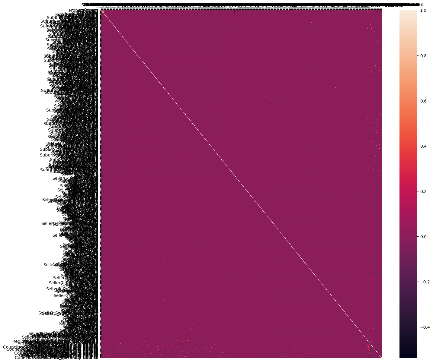
Let’s bifurcate our dataset into train and test dataset
X = dataset.drop('Price', axis=1)
y = dataset['Price']
from sklearn.model_selection import train_test_split
train_X, test_X, train_y, test_y = train_test_split(X, y, test_size=0.3, random_state=2)Let’s train our Linear Regression Model on training dataset and check the accuracy on test set
from sklearn.linear_model import LinearRegression
reg = LinearRegression()
reg.fit(train_X, train_y)LinearRegression()In a Jupyter environment, please rerun this cell to show the HTML representation or trust the notebook.
On GitHub, the HTML representation is unable to render, please try loading this page with nbviewer.org.
LinearRegression()
reg.score(test_X, test_y)0.13853683161649788reg.score(train_X, train_y)0.6827792395792723Here training score is 68% but test score is 13.85% which is very low
Normal Regression is clearly overfitting the data, let’s try other models
Using Lasso (L1 Regularized) Regression Model
from sklearn.linear_model import Lasso
lasso_reg = Lasso(alpha=50, max_iter=100, tol=0.1)
lasso_reg.fit(train_X, train_y)
Lasso(alpha=50, max_iter=100, tol=0.1)In a Jupyter environment, please rerun this cell to show the HTML representation or trust the notebook.
On GitHub, the HTML representation is unable to render, please try loading this page with nbviewer.org.
Lasso(alpha=50, max_iter=100, tol=0.1)
lasso_reg.score(test_X, test_y)0.6636111369404488lasso_reg.score(train_X, train_y)0.6766985624766824Using Ridge (L2 Regularized) Regression Model
from sklearn.linear_model import Ridge
ridge_reg= Ridge(alpha=50, max_iter=100, tol=0.1)
ridge_reg.fit(train_X, train_y)
Ridge(alpha=50, max_iter=100, tol=0.1)In a Jupyter environment, please rerun this cell to show the HTML representation or trust the notebook.
On GitHub, the HTML representation is unable to render, please try loading this page with nbviewer.org.
Ridge(alpha=50, max_iter=100, tol=0.1)
ridge_reg.score(test_X, test_y)0.6670848945194958ridge_reg.score(train_X, train_y)0.6622376739684328We see that Lasso and Ridge Regularizations prove to be beneficial when our Simple Linear Regression Model overfits. These results may not be that contrast but significant in most cases.Also that L1 & L2 Regularizations are used in Neural Networks too