import pandas as pd
df = pd.read_csv("Data/carprices.csv")
df.head()| Mileage | Age(yrs) | Sell Price($) | |
|---|---|---|---|
| 0 | 69000 | 6 | 18000 |
| 1 | 35000 | 3 | 34000 |
| 2 | 57000 | 5 | 26100 |
| 3 | 22500 | 2 | 40000 |
| 4 | 46000 | 4 | 31500 |
We have a dataset containing prices of used BMW cars. We are going to analyze this dataset and build a prediction function that can predict a price by taking mileage and age of the car as input. We will use sklearn train_test_split method to split training and testing dataset
import pandas as pd
df = pd.read_csv("Data/carprices.csv")
df.head()| Mileage | Age(yrs) | Sell Price($) | |
|---|---|---|---|
| 0 | 69000 | 6 | 18000 |
| 1 | 35000 | 3 | 34000 |
| 2 | 57000 | 5 | 26100 |
| 3 | 22500 | 2 | 40000 |
| 4 | 46000 | 4 | 31500 |
import matplotlib.pyplot as pltCar Mileage Vs Sell Price ($)
plt.scatter(df['Mileage'],df['Sell Price($)'])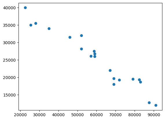
Car Age Vs Sell Price ($)
plt.scatter(df['Age(yrs)'],df['Sell Price($)'])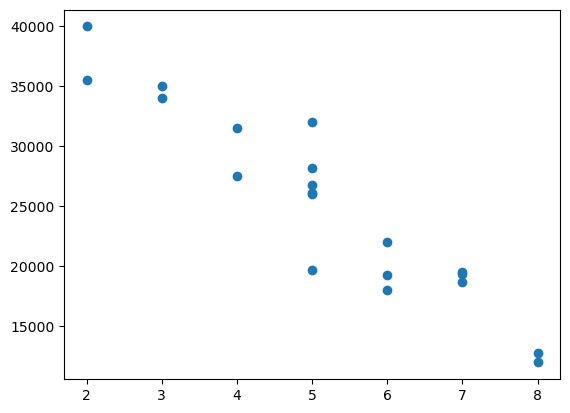
Looking at above two scatter plots, using linear regression model makes sense as we can clearly see a linear relationship between our dependant (i.e. Sell Price) and independant variables (i.e. car age and car mileage)
The approach we are going to use here is to split available data in two sets
<ol>
    <b>
    <li>Training: We will train our model on this dataset</li>
    <li>Testing: We will use this subset to make actual predictions using trained model</li>
    </b>
 </ol>
The reason we don’t use same training set for testing is because our model has seen those samples before, using same samples for making predictions might give us wrong impression about accuracy of our model. It is like you ask same questions in exam paper as you tought the students in the class.
X = df[['Mileage','Age(yrs)']]y = df['Sell Price($)']from sklearn.model_selection import train_test_split
X_train, X_test, y_train, y_test = train_test_split(X,y,test_size=0.3)X_train| Mileage | Age(yrs) | |
|---|---|---|
| 4 | 46000 | 4 |
| 13 | 58780 | 4 |
| 5 | 59000 | 5 |
| 7 | 72000 | 6 |
| 12 | 59000 | 5 |
| 11 | 79000 | 7 |
| 3 | 22500 | 2 |
| 9 | 67000 | 6 |
| 0 | 69000 | 6 |
| 8 | 91000 | 8 |
| 14 | 82450 | 7 |
| 2 | 57000 | 5 |
| 6 | 52000 | 5 |
| 15 | 25400 | 3 |
X_test| Mileage | Age(yrs) | |
|---|---|---|
| 1 | 35000 | 3 |
| 10 | 83000 | 7 |
| 17 | 69000 | 5 |
| 16 | 28000 | 2 |
| 18 | 87600 | 8 |
| 19 | 52000 | 5 |
y_train4 31500
13 27500
5 26750
7 19300
12 26000
11 19500
3 40000
9 22000
0 18000
8 12000
14 19400
2 26100
6 32000
15 35000
Name: Sell Price($), dtype: int64y_test1 34000
10 18700
17 19700
16 35500
18 12800
19 28200
Name: Sell Price($), dtype: int64Lets run linear regression model now
from sklearn.linear_model import LinearRegression
clf = LinearRegression()
clf.fit(X_train, y_train)LinearRegression()In a Jupyter environment, please rerun this cell to show the HTML representation or trust the notebook.
LinearRegression()
X_test| Mileage | Age(yrs) | |
|---|---|---|
| 1 | 35000 | 3 |
| 10 | 83000 | 7 |
| 17 | 69000 | 5 |
| 16 | 28000 | 2 |
| 18 | 87600 | 8 |
| 19 | 52000 | 5 |
clf.predict(X_test)array([34944.44210911, 16905.69832696, 23351.64782019, 38167.41685573,
14300.34495583, 27726.46589653])y_results = pd.DataFrame(clf.predict(X_test))
y_results| 0 | |
|---|---|
| 0 | 34944.442109 |
| 1 | 16905.698327 |
| 2 | 23351.647820 |
| 3 | 38167.416856 |
| 4 | 14300.344956 |
| 5 | 27726.465897 |
y_res = y_results[0].sort_values(ascending=True).reset_index()
y_res.drop('index', axis = 1, inplace=True)
y_res| 0 | |
|---|---|
| 0 | 14300.344956 |
| 1 | 16905.698327 |
| 2 | 23351.647820 |
| 3 | 27726.465897 |
| 4 | 34944.442109 |
| 5 | 38167.416856 |
y_test1 34000
10 18700
17 19700
16 35500
18 12800
19 28200
Name: Sell Price($), dtype: int64y_t = y_test.sort_values(ascending=True).reset_index()
y_t| index | Sell Price($) | |
|---|---|---|
| 0 | 18 | 12800 |
| 1 | 10 | 18700 |
| 2 | 17 | 19700 |
| 3 | 19 | 28200 |
| 4 | 1 | 34000 |
| 5 | 16 | 35500 |
y_t.drop('index', axis = 1, inplace=True)
y_t| Sell Price($) | |
|---|---|
| 0 | 12800 |
| 1 | 18700 |
| 2 | 19700 |
| 3 | 28200 |
| 4 | 34000 |
| 5 | 35500 |
plt.plot(y_t)
plt.plot(y_res)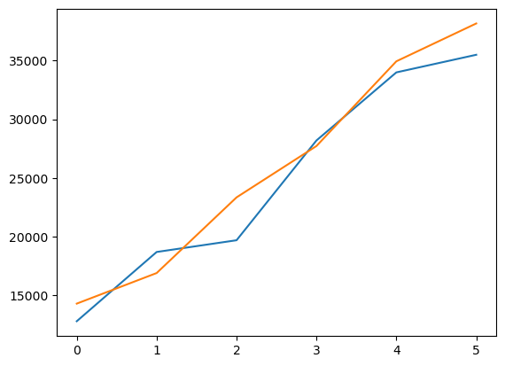
clf.score(X_test, y_test)0.9353054216597069random_state argument
X_train, X_test, y_train, y_test = train_test_split(X,y,test_size=0.3,random_state=10)
X_test| Mileage | Age(yrs) | |
|---|---|---|
| 7 | 72000 | 6 |
| 10 | 83000 | 7 |
| 5 | 59000 | 5 |
| 6 | 52000 | 5 |
| 3 | 22500 | 2 |
| 18 | 87600 | 8 |