Gaussian Mixture Models (GMMs) are a powerful probabilistic tool for modeling a mixture of multiple Gaussian distributions. They are commonly used in unsupervised learning tasks such as clustering, density estimation, and anomaly detection.
Author
Benedict Thekkel
Gaussian Distribution
A Gaussian (or normal) distribution is characterized by its mean (()) and covariance (()). In a (d)-dimensional space, the probability density function of a Gaussian distribution is:
A mixture model represents the presence of subpopulations within an overall population without requiring that an observed dataset identifies the subpopulation to which an individual observation belongs. A Gaussian Mixture Model (GMM) assumes that the data is generated from a mixture of several Gaussian distributions with unknown parameters.
Model Definition
A GMM is defined by the following components:
\(K\): The number of Gaussian components.
\(\pi_k\): The mixing coefficient for component \(k\) with \(\sum_{k=1}^{K} \pi_k = 1\) and \(\pi_k \geq 0\).
\(\mu_k\): The mean vector of the (k)-th Gaussian component.
\(\Sigma_k\): The covariance matrix of the (k)-th Gaussian component.
The probability density function of a GMM is given by:
$ p(x) = _{k=1}^{K} _k , (x _k, _k) $
where \(\mathcal{N}(x \mid \mu_k, \Sigma_k)\) is the Gaussian density for component (k).
Expectation-Maximization (EM) Algorithm
The EM algorithm is used to find the parameters of the GMM that best fit the data. It consists of two main steps:
Expectation (E) Step: Calculate the responsibility that each Gaussian component takes for each data point.
Maximization (M) Step: Update the parameters (π, μ, Σ) to maximize the likelihood of the observed data given these responsibilities.
Applications
GMMs are widely used in:
Clustering: Identifying groups in data.
Anomaly Detection: Detecting outliers as points with low probability under the model.
Density Estimation: Estimating the underlying distribution of data.
Implementation
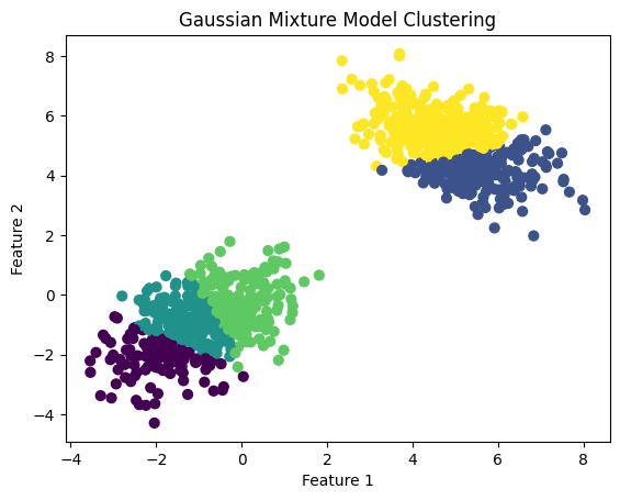
import numpy as npfrom sklearn.mixture import GaussianMixtureimport matplotlib.pyplot as plt# Generating sample datanp.random.seed(0)n_samples =500# Generate random samples from two different Gaussian distributionsX = np.vstack([np.random.multivariate_normal(mean=[-1, -1], cov=[[1, 0.5], [0.5, 1]], size=n_samples), np.random.multivariate_normal(mean=[5, 5], cov=[[1, -0.5], [-0.5, 1]], size=n_samples)])# Fit the GMM modelgmm = GaussianMixture(n_components=5, covariance_type='full')gmm.fit(X)# Predict the labels for the data pointslabels = gmm.predict(X)# Plotting the resultsplt.scatter(X[:, 0], X[:, 1], c=labels, s=40, cmap='viridis')plt.title('Gaussian Mixture Model Clustering')plt.xlabel('Feature 1')plt.ylabel('Feature 2')plt.show()
Key Considerations
Number of Components (K): Choosing the right number of components is crucial and can be done using methods like the Bayesian Information Criterion (BIC) or the Akaike Information Criterion (AIC).
Initialization: The EM algorithm is sensitive to initialization. Using multiple initializations and choosing the best model can help.
Covariance Type: GMMs allow different covariance structures (‘full’, ‘tied’, ‘diag’, ‘spherical’). The choice depends on the nature of the data.
Advantages and Disadvantages
Advantages: - Flexibility: GMMs can model any continuous data distribution, given enough components. - Probabilistic Model: Provides a probabilistic framework that can be used for soft clustering.
Disadvantages: - Computational Complexity: EM algorithm can be computationally expensive, especially for large datasets. - Local Optima: The EM algorithm may converge to a local optimum, making the initialization important.