import pandas as pd
from fastai.vision.all import *Decision Tree
A bunch of if statement placed at low point of entropy
Advantages of CART
- Simple to understand, interpret, visualize.
- Decision trees implicitly performvariable screening or feature selection.
- Can handle both numerical and categorical data. Can also handle multi-output problems.
- Decision trees require relatively little effort from users for data preparation.
- Nonlinear relationships between parameters do not affect tree performance.
Disadvantages of CART
- Decision-tree learners can create over-complex trees that do not generalize the data well. This is called overfitting.
- Decision trees can be unstable because small variations in the data might result in a completely different tree being generated. This is called variance, which needs to be lowered by methods like bagging and boosting.
- Greedy algorithms cannot guarantee to return the globally optimal decision tree. This can be mitigated by training multiple trees, where the features and samples are randomly sampled with replacement.
- Decision tree learners create biased trees if some classes dominate. It is therefore recommended to balance the data set prior to fitting with the decision tree.
path = Path('Data')
name = 'salaries.csv'
df = pd.read_csv(path/name)
df.head()| company | job | degree | salary_more_then_100k | |
|---|---|---|---|---|
| 0 | sales executive | bachelors | 0 | |
| 1 | sales executive | masters | 0 | |
| 2 | business manager | bachelors | 1 | |
| 3 | business manager | masters | 1 | |
| 4 | computer programmer | bachelors | 0 |
inputs = df.drop('salary_more_then_100k',axis='columns')target = df['salary_more_then_100k']from sklearn.preprocessing import LabelEncoderle_company = LabelEncoder()
le_job = LabelEncoder()
le_degree = LabelEncoder()inputs['company_n'] = le_company.fit_transform(inputs['company'])
inputs['job_n'] = le_job.fit_transform(inputs['job'])
inputs['degree_n'] = le_degree.fit_transform(inputs['degree'])inputs| company | job | degree | company_n | job_n | degree_n | |
|---|---|---|---|---|---|---|
| 0 | sales executive | bachelors | 2 | 2 | 0 | |
| 1 | sales executive | masters | 2 | 2 | 1 | |
| 2 | business manager | bachelors | 2 | 0 | 0 | |
| 3 | business manager | masters | 2 | 0 | 1 | |
| 4 | computer programmer | bachelors | 2 | 1 | 0 | |
| 5 | computer programmer | masters | 2 | 1 | 1 | |
| 6 | abc pharma | sales executive | masters | 0 | 2 | 1 |
| 7 | abc pharma | computer programmer | bachelors | 0 | 1 | 0 |
| 8 | abc pharma | business manager | bachelors | 0 | 0 | 0 |
| 9 | abc pharma | business manager | masters | 0 | 0 | 1 |
| 10 | sales executive | bachelors | 1 | 2 | 0 | |
| 11 | sales executive | masters | 1 | 2 | 1 | |
| 12 | business manager | bachelors | 1 | 0 | 0 | |
| 13 | business manager | masters | 1 | 0 | 1 | |
| 14 | computer programmer | bachelors | 1 | 1 | 0 | |
| 15 | computer programmer | masters | 1 | 1 | 1 |
inputs_n = inputs.drop(['company','job','degree'],axis='columns')inputs_n| company_n | job_n | degree_n | |
|---|---|---|---|
| 0 | 2 | 2 | 0 |
| 1 | 2 | 2 | 1 |
| 2 | 2 | 0 | 0 |
| 3 | 2 | 0 | 1 |
| 4 | 2 | 1 | 0 |
| 5 | 2 | 1 | 1 |
| 6 | 0 | 2 | 1 |
| 7 | 0 | 1 | 0 |
| 8 | 0 | 0 | 0 |
| 9 | 0 | 0 | 1 |
| 10 | 1 | 2 | 0 |
| 11 | 1 | 2 | 1 |
| 12 | 1 | 0 | 0 |
| 13 | 1 | 0 | 1 |
| 14 | 1 | 1 | 0 |
| 15 | 1 | 1 | 1 |
import matplotlib.pyplot as plt
import numpy as npnp.random.seed(42)
n_points = len(inputs_n)
x = np.random.rand(n_points)
y = np.random.rand(n_points)
z = np.random.rand(n_points)inputs_n['company_n'] += (x-0.5)/10
inputs_n['job_n'] += (y-0.5)/10
inputs_n['degree_n'] += (z-0.5)/10# Create a 3D scatter plot
fig = plt.figure()
ax = fig.add_subplot(111, projection='3d')
ax.set_xlabel('degree_n')
ax.set_ylabel('job_n')
ax.set_zlabel('company_n')
scatter = ax.scatter(inputs_n['degree_n'],
inputs_n['job_n'],
inputs_n['company_n'],
c=target,
cmap='viridis',
marker='+')
# Adding a color bar to show the mapping of colors to values in 'color_column'
cbar = fig.colorbar(scatter, ax=ax)
cbar.set_label('Color Column')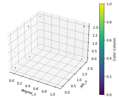
target0 0
1 0
2 1
3 1
4 0
5 1
6 0
7 0
8 0
9 1
10 1
11 1
12 1
13 1
14 1
15 1
Name: salary_more_then_100k, dtype: int64from sklearn import treemodel = tree.DecisionTreeClassifier()
model.fit(inputs_n, target)DecisionTreeClassifier()In a Jupyter environment, please rerun this cell to show the HTML representation or trust the notebook.
On GitHub, the HTML representation is unable to render, please try loading this page with nbviewer.org.
DecisionTreeClassifier()
model.score(inputs_n,target)1.0from sklearn.tree import export_graphvizFEATURE_NAMES = ['company_n', 'job_n', 'degree_n']
export_graphviz(model, './Data/salary.dot', feature_names = FEATURE_NAMES)!dot -Tpng ./Data/salary.dot -o ./Data/salary.pngimport matplotlib.pyplot as plt
import cv2 as cvimg = cv.imread('./Data/salary.png')
plt.figure(figsize = (20, 20))
plt.imshow(img)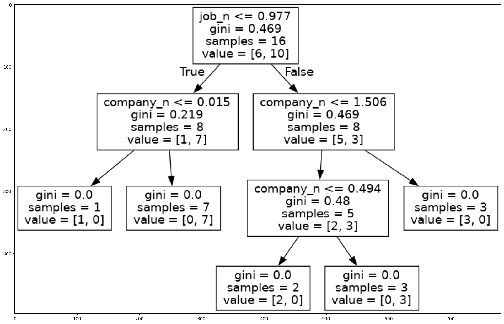
Predict
model.predict([[2,1,0]])/home/ben/mambaforge/envs/cfast/lib/python3.11/site-packages/sklearn/base.py:464: UserWarning: X does not have valid feature names, but DecisionTreeClassifier was fitted with feature names
warnings.warn(array([0])model.predict([[2,1,1]])/home/ben/mambaforge/envs/cfast/lib/python3.11/site-packages/sklearn/base.py:464: UserWarning: X does not have valid feature names, but DecisionTreeClassifier was fitted with feature names
warnings.warn(array([0])